
 CC-BY 4.0
Introduction
Fabric is made of the orientation and dip of elongated objects (Bertran et al., 1997; Bertran & Lenoble, 2002; Lenoble & Bertran, 2004). It is a statistic (i.e. it needs as much measurements as possible) that enables the identification of sedimentary processes involved in the formation of the deposits (Bertran et al., 1997; Bertran & Lenoble, 2002; Lenoble & Bertran, 2004) and their impact on archaeological assemblages (Isaac, 1967; Schick, 1986; Thomas et al., 2019). Objects abandoned by prehistoric people can be considered as sedimentary particles and are affected by natural processes (Schiffer, 1983). As geological particles are often not elongated enough, analysis of the fabric of sedimentary deposits often depends mainly on archaeological material (bones and lithics). This makes it possible to identify the sedimentary processes to which they were subjected and to discuss their degree of spatial reorganization. When possible, distinguishing sedimentary particles from archaeological objects in the fabric analysis could allow to test whether these two populations were affected by different processes (e.g. the fabric of an undisturbed occupation covered by deposits from a minor flood should reveal a distinct fabric from that of the alluvial pebbles on which it rests).
One of the first archaeological application probably dates to the experiments carried out by the South African G. Isaac (1967) on the shores of Lake Magadi in Kenya. G. Isaac wanted to explain the role played by hydrological processes on the bone accumulations found in the Great Rift Valley. In November 1964, he placed several concentrations of experimental material near a river branch. A few months later, heavy rains had reactivated the valley’s rivers. In addition to the displacement or even loss of all or part of the material, G. Isaac revealed a reorientation that was mainly perpendicular and, to a lesser extent, parallel to the orientation of flow, with a slight upstream dip. Since G. Isaac’s pioneering work, there has been an abundant literature devoted to the analysis of fabrics (Benn, 1994; Lenoble & Bertran, 2004; McPherron, 2018) allowing this method to be increasingly performed on archaeological sites.
Numerical methods have been developed to measure the orientation and dip of objects in the field (McPherron, 2005; Discamps et al., 2024) or from field archives such as plans and photos (de la Torre & Benito-Calvo, 2013; Sánchez-Romero et al., 2016).
Two main families of statistical method are commonly used to characterize the fabric of a given assemblage (Bertran & Lenoble, 2002; McPherron, 2018; de la Torre et al., 2021). The first methods focus on the orientation only and aim to test the null hypothesis of a random orientation of objects through several statistical tests (Krumbein, 1939; Curray, 1956; Rao, 1967).The second statistical method takes into account object orientation and dip. Three normalized eigenvalues (E1, E2 and E3) are calculated from the cosine formed by the axis of the artifact with the three axes of space (Watson, 1966). Woodcock (1977) and Benn (1994) indices are used to describe the fabric shape. Several authors (e.g. Bertran et al., 1997; Bertran & Lenoble, 2002; Lenoble & Bertran, 2004) built models to compare the fabric of archaeological assemblages to natural sedimentary processes and human processes (i.e. fabric of knapping spots). The null hypothesis of an absence of perturbation is a fabric shape compatible with that of experimental knapping spots. These methods are described in the Mathematics section of this article.
Several software allow data processing, some of which are not freely accessible, do not allow spatial exploration of the data or do not offer interfaces to facilitate the task of non-programmer users (McPherron, 2018). The following sections explain all the selected approaches and our proposals for processing the fabrics thanks to fabryka, from taking measurements in the field, through the statistical methods and graphical modes of representation used in the application (Figure 1).
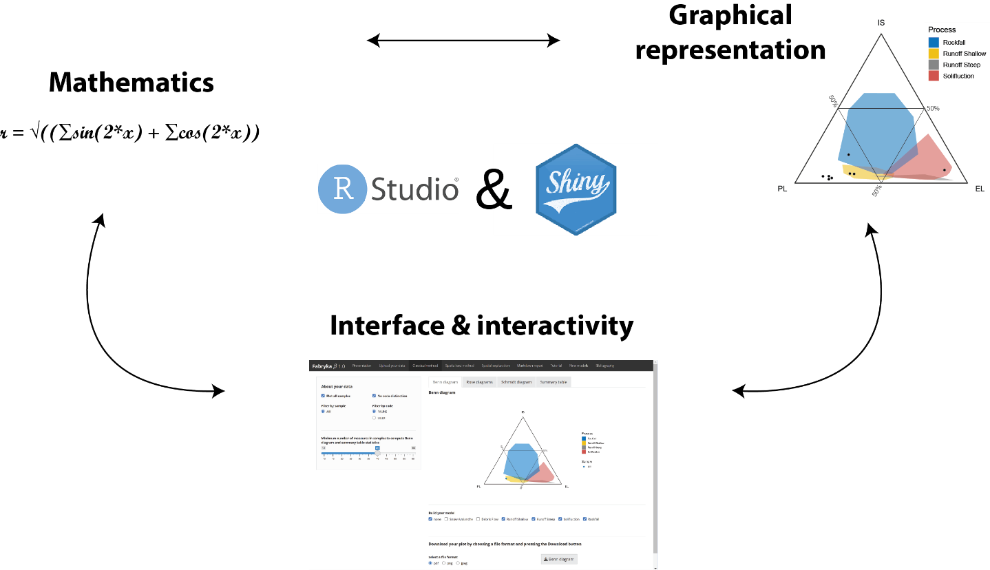
Figure 1 - fabryka creation scheme and organization of the article.
Field data acquisition
During excavation, the orientation and dip of elongated remains (i.e. a > 2 * b and with a > 2 cm) is measured on a representative set of artefacts or on the whole assemblage. The orientation (= bearing) of the lowest point is measured in the range [0; 360[ with North as the reference (i.e. orientation = 0°). The dip (= plunge) is measured in the range [0; 90] with horizontal as a reference. The orientation [0; 360[ can be converted into axial data measured in the range [0; 180[ by subtracting 180° from the measurements in the range [180; 360].
Traditionally, the azimuth of the principal axis of an object is measured using a compass considering that the point with the lowest altitude indicates the orientation of the vector. The dip is measured using an inclinometer. The aim is to measure the orientation and dip of the elongaton axis of of objects ignoring its shape. To do this, the measuring device must be placed parallel to the elongation axis of the object. Measuring the fabric from its imprint or visible surface is biased by its shape, making impossible to assess its true dip. Since the theodolite was introduced to excavations in the 1990s, the fabrics is sometimes measured by recording the coordinates of the ends of objects (McPherron, 2005). In the latter case, the rules of trigonometry are applied to convert the pair of coordinates into orientations and dips.
Recently, speleologist have created a digital inclinometer (Leica DistoX310 modified to DistoX2; https://paperless.bheeb.ch/) which can be used to measure fabrics (Discamps et al., 2024). The device stores and associates data with the order of measurement. When the device is tilted downwards, the orientation of the lowest point is measured and, the recorded dip is negative. When the device is tilted upwards, the orientation of the highest point is recorded, and the dip is positive. To obtain data that is suitable for statistical analysis, in the first case the absolute value of the dip must be retained. In the second case (i.e. positive dip), if the measured orientation is in the interval [0; 180], 180° must be added to the orientation, and if the measured orientation is in the interval ]180; 360], 180° must be subtracted from the orientation.
When possible, preferring the use of a digital inclinometer avoids many errors during measurement and data recording. On the other hand, for the reasons given above, the use of a theodolite to measure fabrics is not recommended as it results in inaccurate dip measurements. As well, measuring orientations and dip in sections leads to sampling biases.
A sample corresponds to all the orientation and dip measurements taken within a Lithostratigraphic Unit (LU) or a pedostratigraphic unit. These units seem to be the most coherent entity which needs to be explored because they are defined according to geological criteria, which a priori guarantee a certain coherence in terms of the formation dynamics we are seeking to approach. In fabryka, analysis is constrained within samples unless the user decides otherwise in the spatial exploration panel.
Mathematics
Classical method
Two main statistical family methods are used:
The first considers the orientation only. The calculation of the Vector Magnitude \(L\) (expressed as a percentage) by Curray’s (1956) formula tests the hypothesis of a unimodal distribution of orientations. If the \(p\) value returned by the Rayleigh test is less than the threshold of 0.05, the null hypothesis of a random sampling from a uniform distribution is rejected. The formula for calculating the Vector Magnitude \(L\) is as follows:
\(L = \frac{r*100}{n}\)
With:
\(r = \sqrt{\sum_{i = \alpha}^{n}\sin(2\alpha) + \sum_{i = \alpha}^{n}\cos(2\alpha)}\)
Where \(n\) is the number of measures and \(\alpha\) is the axial data (0 to 180°).
The Rayleigh test is performed thanks to the formula:
\(p = e^{\left( - \left( n*L^{2} \right) \right)*10^{-}4}\)
The method consisting of doubling the value of the axial angles before calculating the Vector Magnitude L and the Rayleigh test, as proposed by Krumbein (1939), tests the hypothesis of a bimodal distribution with a period of 90°. The hypothesis of a 90° period bimodal distribution of a sample of orientations is retained when p <0.05 (Curray, 1956). The sensitivity of the Rayleigh test to the sample size n prevents samples from being compared with each other when n varies (Curray, 1956; Bertran & Lenoble, 2002). For example, when the Vector Magnitude \(L\) is 25%, the Rayleigh test gives \(p - values\) below a critical threshold of 0.05 for series with more than 50 measurements (Figure 2).
The Rao (1967) spacing test assesses the uniformity of circular data. It determines whether the data show significant directionality (i.e. the null hypothesis is a uniform distribution). It is widely used to detect multimodal directionality.
The second considers the orientation and dip of the objects. The normalised eigenvalues E1, E2 and E3 are calculated from the cosine formed by the axis of the objects with the three axes of space (Watson, 1966).
The fabric shape can be described by calculating the ratios \(r1\) = ln(E1/E2), \(r2\) = ln(E2/E3) and \(K\) = r1/r2 (Woodcock, 1977). When 0 < \(K\) < 1, the fabric is planar. When 1 < \(K\) < \(+ \infty\), the fabric is linear. The parameter \(C\) = ln(E1/E3) is a measure of the strength of the preferred orientation (Woodcock, 1977). These indices can be plotted into a Woodcock diagram.
The Benn indices (Benn, 1994) describe the fabric shape of a sample and can be plotted in a ternary diagram (i.e. Benn diagram). The elongation index EL is equal to \(1 - (E2/E1)\) and the isotropy index \(IS\) is \(E3/E1\). When \(EL\) is high, the axes of the objects are grouped around an orientation. When \(IS\) is high, the fabric is said to be isotropic meaning the axes of the objects are uniformly distributed in all directions. Finally, when the value \(1 - EL - IS\) is high, the fabric is said to be planar, with the axes of the objects grouped around a plane.
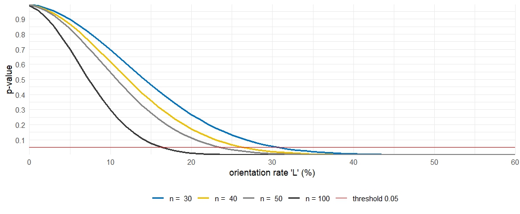
Figure 2 - Evolution of the p-value returned by the Rayleigh test as a function of the Vector Magnitude ‘L’ and the sample size ‘n’.
Spatialised method
To distinguish different statistical populations, a spatial method proposed by McPherron (2018) is used. Thanks to this method it is possible to calculate the Benn indices and the Vector Magnitude \(L\) (formula (3) modified from McPherron (2018) R script) for each remains, and its \(n\) nearest neighbors in 3 dimensions (McPherron (2018) R script, modified, formula (4)). The analysis of the fabric as proposed by McPherron (2018) has the advantage of spatialising the measurements. It is possible to localize the statistical signal of fabrics by varying the number of measurements sampled to calculate the Benn indices. The choice of about 40 to 60 measurements (each remain and its 40 to 60 nearest neighbors) to calculate the Benn indices allows local particularities to be observed, and above all, it allows the Rayleigh test to be carried out in its field of application (stability of the test between around 40 to 50 measurements after Bertran & Lenoble (2018)).
By avoiding the instability of the Rayleigh test, the rejection rate \(Tr\) of the null hypothesis provides a more reliable description of the distribution of orientations in a sample. In addition, it allows comparisons between samples despite varying sample size. The rejection ratio \(Tr\) is performed thanks to the formula:
\(Tr = \frac{(n\ times\ p.value < 0.05)*100}{n}\)
Graphical representation
Several methods of representation are used. Rose diagrams summaries the orientation and dip measurements for each sample. Benn indices are projected in a Benn diagram and measures (orientation and dip) are projected into Schmidt diagrams. These figures are available for both ‘classical’ and ‘spatialised’ methods.
As submited by McPherron (2018), a spatial investigation of the fabric is proposed in a dedicated panel. Benn (1994) indices calculated for each spatial series of remains are projected within a Benn diagram in which each pole (isotropic, linear, and planar) is colored respectively in red, green and blue. The RGB color code is reused to materialize the fabric of the remains on spatial projections (plan and section views) of the material along the axes of the excavation grid.
Interface and user interactivity
The next sections provide a description and a tutorial of fabryka. All the figures in this section were produced using the example data set provided in the application (i.e. “Case 3: Angles from DistoX2 with coordinates”).
Upload data
The simplest method to upload data in the application is to name the column directly, as shown in the example files. Enter your data in a csv file, adding the columns ‘id’, ‘code’ and ‘sample’. If the columns don’t exist, fill them in with the same letter. By doing so, you do not need to select your variables in the main panel. The application correctly reads the data file directly.
First, upload your .csv file in the left sidebar panel (Figure 3A). Pay attention to your decimal and column delimiters (Figure 3B and 3C).
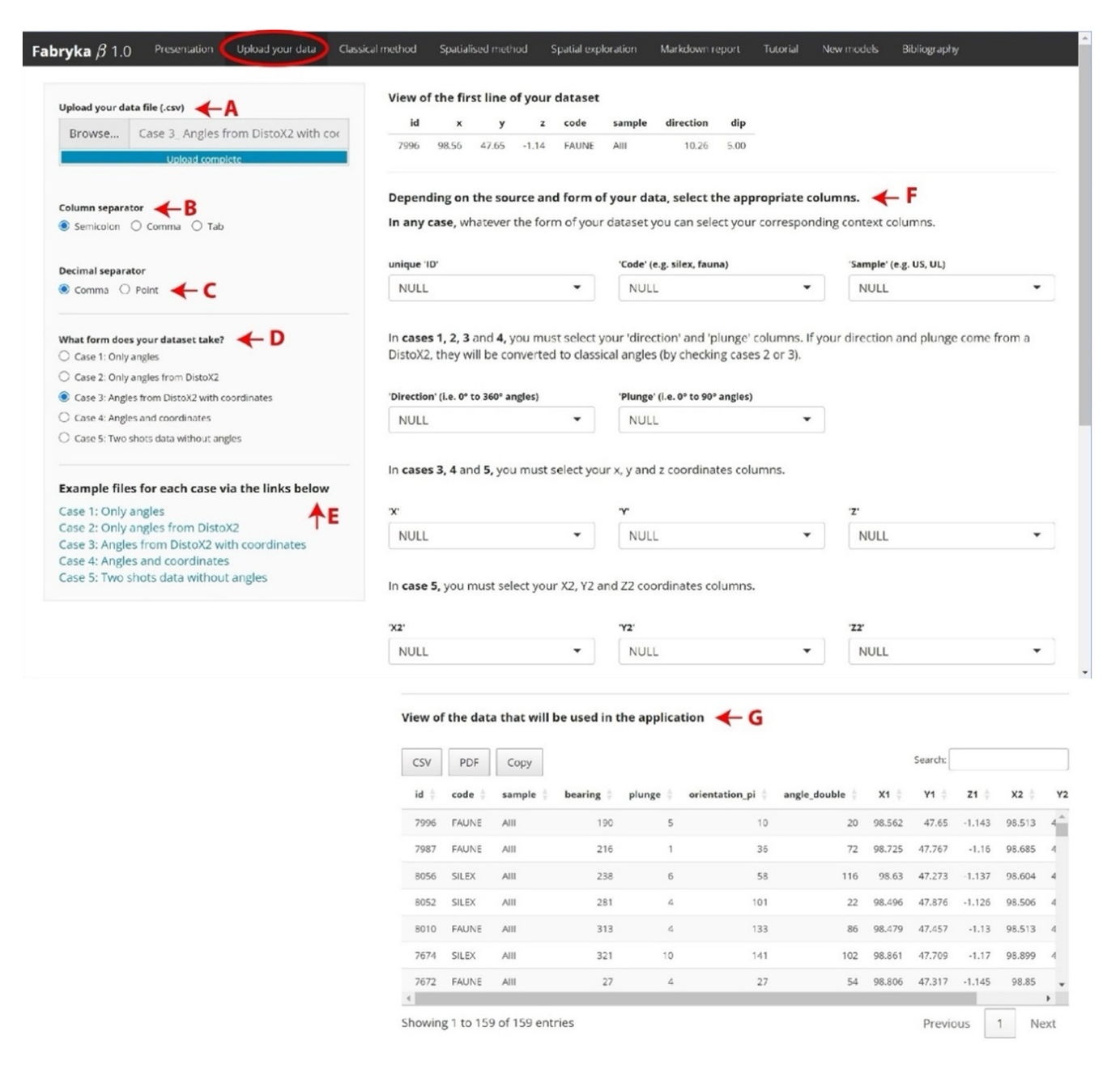
Figure 3 - A. Browse your .csv file, B. choose your column separator, C. choose your decimal separator, D. check the right form of your dataset, E. to do so, have a look of example files, F. select the column needed in the application, G. a new dataset with new columns appears, you are ready to explore your data.
fabryka supports three angle measurement methods:
angles taken with a compass and an inclinometer.
angles taken with a DistoX2.
angles taken with two shots at the total station.
Five cases (i.e. forms of data) are covered by the application (Figure 3D):
check ‘Case 1: Only angles’ if you have in your data set the columns ‘id’, ‘sample’, ‘code’, ‘orientation’ and ‘dip’.
check ‘Case 2: Only angles from DistoX2’ if you have in your data set the same columns that above but your data comes from a DistoX2 and needs to be converted.
check ‘Case 3: Angles from DistoX2 with coordinates’ if you have in your data set the same columns that above (Case 2, data from DistoX2) with a single set of coordinates (x, y, z).
check ‘Case 4: Angles and coordinates’ if your data has the same form that above (Case 3) but is coming from a compass and an inclinometer.
check ‘Case 5: Two shots data without angles’ if you have the columns ‘id’, ‘sample’, ‘code’ and the angles have been measured with a total station (i.e. two shots data).
According to your method of angle measurement and the presence of coordinates you must select the right case. Please refer to the example files in the left side bar panel (Figure 3E). It contains a data set coming from the Lower shelter of Le Moustier (Thomas et al., 2019; Texier et al., 2020). The example files directly contain the right column names. You can use them directly in the application. Whatever the names of the columns in your file, you can select the appropriate columns in the column selector (Figure 3F). Please keep only complete lines (i.e. no empty modalities, so no line without a fabric measurement). When a data table with new columns appears below the column selector, you are ready to use the application.
If your data comes from a DistoX2, the columns ‘orientation’ (= ‘bearing’, i.e. 0 to 360°) and ‘dip’ (= ‘plunge’) are automatically corrected in the new table. Whatever the form of your data set, two new columns ‘orientation_pi’ (0 to 180° angles) and ‘angle_double’ (see Krumbein 1939) appear. If the angles were measured using a total station (i.e. two shots data or 2 by 2 coordinates of plotted pieces refits), the orientation and the dip are calculated. If only one set of coordinates is provided with angles, a second set of coordinates is calculated and displayed in the new table (Figure 3G). You can download the new data by clicking the ‘copy’, the ‘csv’ or the ‘pdf’ buttons.
Classical method
The classical method (Figure 4) can be computed for all sources of data and absence/presence of coordinates (i.e. all cases described above). This panel includes:
Benn diagrams with possible integration of Bertran & Lenoble (2002) model (Figure 4D).
Rose diagrams for axial data and dip (Figure 4G).
Schmidt diagrams (Figure 4H).
Woodcock diagrams.
Summary data table with Benn indices, additional statistics, and orientation statistical tests.
In this last table (Figure 4I):
\(N\) stands for number of measures in the samples.
\(E1\), \(E2\) and \(E3\) are the eigenvalues (Watson, 1966). They correspond to the sum of the cosines formed by the axis of the objects and the three axes of the space. They are used to compute the Benn indices.
\(IS\) and \(EL\) are the Benn indices ratios standing respectively for, ‘isotropy’ with \(IS = E3/E1\) and ‘elongation’ with \(EL = 1 - (E2/E1)\) (Benn, 1994).
\(K\) and \(C\) are the Woodcock (1977) indices.
\(L\) is the Vector Magnitude (strength of the preferred orientation) and \(R.p\) is the p-value result of the Rayleigh test.
\(L.double\) and \(R.p.double\) are the same statistics that above for double angles (Krumbein, 1939).
\(Rao_{p}\) is the p_value of the Rao (1967) test.
You can control the data you plot and the data appearing in the figures and the summary data table by changing the checkboxes filters (‘filter by sample’ and ‘filter by code’) and the slider (i.e. minimum number of measures) in the left sidebar panel (Figure 4A, 4B and 4C).
Certain geological processes can have a different impact on objects depending on their physical properties (e.g. silex versus bones in a water flow as in the example files provided where bones have a strong preferential orientation and are much more ‘linear’ in the Benn diagram (Thomas et al., 2019; Texier et al., 2020)). The natural processes models that you can add to the Benn diagram are calculated using data mainly from (Bertran et al., 1997, 2006; Bertran & Lenoble, 2002; Lenoble & Bertran, 2004). You will find the reference model data (with corresponding literature references) which is used in the application in the ‘Model reference data’ subpanel. In the rose diagram, axial data is considered (and not orientations) as the Rayleigh test is perform on axial data (Curray, 1956) in the summary table. You can download all the figures by selecting a file format (.pdf, .jpeg and .png) and pressing the ‘download’ button (Figure 4E and 4F).
Spatialised method
This panel includes (Figure 5):
Benn diagrams with Benn indices computed with nearest neighboring points (McPherron, 2018).
Spatial projections of the points according to their fabric shape.
Summary data tables with orientation statistical tests, one at the scale of each spatial series (each object and its \(n\) nearest neighboring points = one row) and one at the scale of the sample (Figure 5F and 5G).
A table similar to the one done in the Classical method is proposed and contains the same statistics.
At the spatial series scale (i.e. each points and \(n\) neighbors), statistics are provided in a table (Spatial series data table subpanel) with the Benn indices, the orientation rates \(L\), \(L.double\) and \(p - values\) returned by the Rayleigh tests. At the sample scale, mean and standard deviations values of Benn indices, mean \(L\) and its corresponding Rayleigh tests means (mean values of all spatial series in the sample) and rejections ratios \(Tr\) (formula (4)) are given in the subpanel ‘Summary table of samples’.
In the projections, the orientation of the objects can be materialized by sticks (by unchecking the corresponding box in the left sidebar panel, Figure 5D) which color is representative of the fabric of the series formed by the object and its \(n\) nearest neighbors. You can also add orthophoto in the background of projections (Figure 5E). In the left sidebar panel, you can control the samples considered in the analysis by selecting the sample explored or by distinguishing the code used (e.g. flint versus bone, Figure 5A and 5B). You can also use the slider to change the number of neighbors searched for around each point (Figure 5C). Be careful, this will alter the results obtained in the Benn diagram and Rayleigh tests.
Spatial exploration
This panel includes (Figure 6):
A spatial exploration of your data starting from a Benn diagram
A spatial exploration of your data starting from the spatial projections (Figure 6J)
Summary data tables with orientation statistical tests (Figure 6I and 6K).
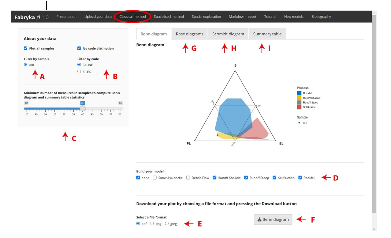
Figure 4 - A. filter by sample, B. if you want to filter by codes, uncheck ’no code distinction’, C. manage the minimum sample size to perform analysis, D. build your model thanks to Bertran and Lenoble (2002) data, E. and F. download figures by selecting a file format and pressing the ’download’ button, G. Rose diagrams subpanel, H. Schmidt diagram subpanel, I. Summary table with additional statistics.
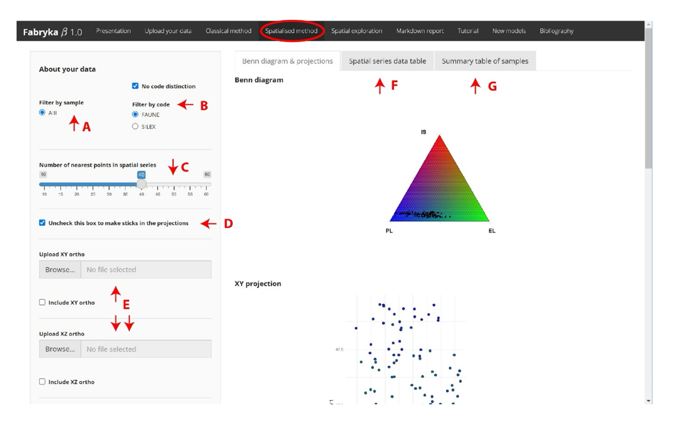
Figure 5 - A. filter by sample, B. if you want to filter by code, uncheck ’no code distinction’, C. choose the n nearest neighbors to perform the statistics, D. make sticks in spatial projections, E. upload a georeferenced orthophoto and check ’include’ orthophoto to display it, F. new dataset at the spatial series scale, G. summary table at the sample scale.
In this panel, you can perform a spatial analysis of your data starting from a Benn diagram or from projections. In both cases, you need to select the data you want to explore more locally in a new analysis. From the projections, you can select the points you want to explore directly. In the Benn diagram, you need to select the lasso selector (Figure 6D). Pay attention to the number of points selected and check that the new sample contains enough points to carry out the new analysis. If this is not the case, you can lower the slider in the left sidebar panel to perform the analysis with fewer neighbors (Figure 6E). You can download the new samples you have selected with spatial statistics from the corresponding subpanels (Figure 6I and 6K).
Tutorial
The ‘Tutorial’ panel contains a summary of the mathematics, statistics and methods used in fabryka and a short tutorial directly accessible from the application.
New models
The ‘spatialised’ method generates often more linear fabrics in comparison with the ‘classical’ method. This can be explained by the fact that objects that are close in space are more likely to resemble each other than objects that are further in space. A difference between global fabric (“classical method”, i.e. one point per sample) and spatialised fabric (series of n neighbors) in Benn diagrams marks a spatial heterogeneity that needs to be explored.
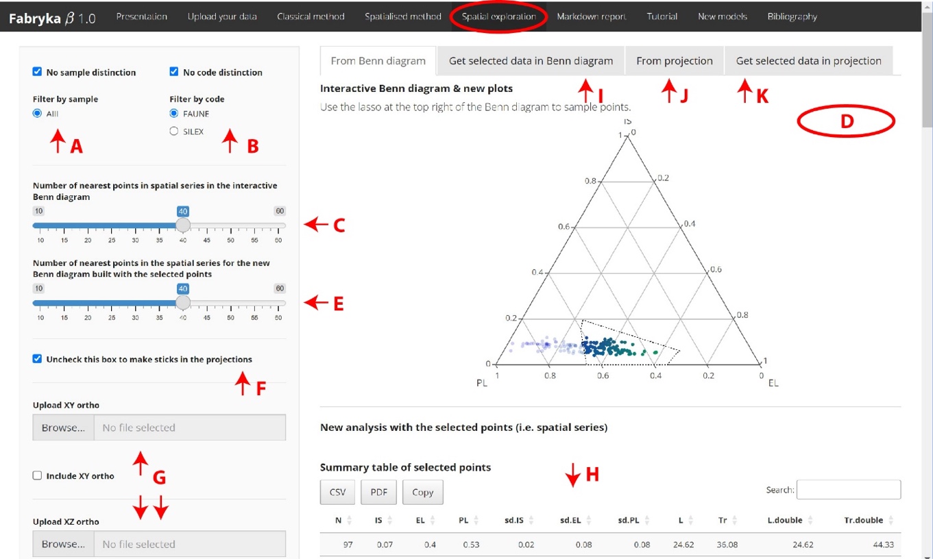
Figure 6 - A. if you want to filter by sample, uncheck ’No sample distinction’ B. if you want to filter by code, uncheck ’no code distinction’, C. choose the n nearest neighbors to perform the statistics (first Benn diagram), E. choose the n nearest neighbors to perform the statistics on the sampled data (second Benn diagram), F. make sticks in spatial projections, G. you can upload a georeferenced orthophoto and check ’include’ orthophoto to display it, H. a new spatial exploration of the fabric is performed, I. new dataset at the selected spatial series scale, I. a similar spatial exploration is possible from the projections, K. new dataset at the selected spatial series scale.
Also, the structure of the point pattern is evocative of its fabric. Thus, the dispersion of the points depends on the shape of the fabric. Two extremes appear: the most isotropic samples are those with the most dispersed point patterns (i.e. the standard deviations are high) while the most linear samples are those with the least dispersed point patterns. Planar samples highlight point patterns with intermediate dispersion. The explanation of this phenomenon is intuitive: the more similar the fabrics of objects are, the closer they are in the Benn diagram and the more linear they are. To reflect this phenomenon, the standard deviations of the Benn indices are calculated and aim to describe the dispersion point patterns in the Benn diagrams.
Global planar or isotropic fabrics can sometimes mask local anisotropy. Within certain samples, groups of objects form a dense cluster in the point pattern. This is expressed either by a locally more linear fabric, or by a planar fabric with a strong bimodal orientation.
For the reasons given above, we wish to create new models that considered the particularities of the spatial method. A panel was therefore set up to collect new data describing the fabric of sedimentary processes in order to build a new “spatialised” reference model (cf. the “classical” model proposed by Bertran & Lenoble (2002)). This work is in progress. This panel will be updated in the next version of the application.
Contributors
The contributors panel aims at citing all contributors of this project.
Data, scripts, code, and supplementary information availability
use fabryka online: https://marchaeologist.shinyapps.io/fabryka/
source code: https://github.com/marchaeologist/fabryka/tree/main
report bugs or any request: https://github.com/marchaeologist/fabryka/issues
github repository of fabryka (Thomas, 2025): https://doi.org/10.5281/zenodo.15909666
If you are preparing a mission in a field without Internet access:
Install R (https://www.r-project.org/) and Rstudio Desktop (https://posit.co/download/rstudio-desktop/).
Clone the fabryka repository from GitHub: https://github.com/marchaeologist/fabryka or download the code in “Code” and “Download ZIP” at the same address. Unzip the folder. This will give you the latest version of the source code.
Open fabryka.Rproj
If you are using the application for the first time, you have to install several packages used in the application. Lists of all these packages and dependencies are available in a DESCRIPTION file and a DEPENDECIES file in the github repository. To install fabryka packages and dependencies, copy and paste the following code lines into the R console:
fabryka_packages = c(“shiny”, “dplyr”,”ggplot2”,”plotly”, “ggsci”, “ggtern”, “circular”,
“CircStats”, “Ternary”, “RStoolbox”, “shinyjs”, “rmarkdown”,
“shinythemes”, “ggalt”, “DT”, “raster”)
is_installed = sapply(fabryka_packages, require, character.only=T)
sapply(fabryka_packages[!is_installed], install.packages)
The application can be launched by opening the app.R file in the main folder and pressing “Run App” or by running the following commands:
pkgload::load_all(“.”)
fabryka()
Acknowledgements
The writing of the script was greatly facilitated by the work published by Shannon McPherron (2018). It includes some functions published by the author, with a few modifications. This work benefited from discussions with Jean-Pierre Texier, Arnaud Lenoble, Pascal Bertran, Thomas Perrin and Dominique Todisco on issues related to site formation processes. The reference data used to build the models of the classical method were collected by Pascal Bertran throughout his career. Pascal Bertran provided us with all these data in order to feed the application. The development of the application also benefited from the help of Rémi Lemoy, François Baleux and Victor Baleux on mathematical issues. A first version of the application was tested by Emmanuel Discamps and Aurélien Royer. This project is supported by the “Service Valorisarion de la Recherche” of the University Toulouse Jean Jaurès. Preprint version 3 of this article has been peer-reviewed and recommended by PCI Archaeology (https://doi.org/10.24072/pci.archaeo.100611; Bertran, 2025). Comments made by Pascal Bertran, recommender of this article, and, by Frédéric Santos, Nicolas Frerebeau and Alfonso Benito-Calvo, reviewers of this article, considerably improved the manuscript and the application. I would like to thank all these researchers for their advice.
Funding
This research was funded by the Service Valorisation de la Recherche of Toulouse - Jean Jaurès University.
Conflict of interest disclosure
The authors declare that they comply with the PCI rule of having no financial conflicts of interest in relation to the content of the article.
Note
The ‘Bibliography’ panel in the application contains the references cited in the application. This article contains the same bibliography with some additional references.