
 CC-BY 4.0
Introduction
Statistical tests should be robust to common violations of distributional assumptions (Huber & Ronchetti, 2009; Loh, 2024; Morgenthaler, 2007; Wilcox, 2013). Such violations should not distort the binary decisions informed by a test—for instance, the provisional acceptance of a hypothesis or the grounding of future research on an observed effect. In the falsificationist tradition, rigid frequentist hypothesis testing adheres to prespecified error rates: Type I errors, rejecting a true null hypothesis and producing a false positive, and Type II errors, not rejecting a false null hypothesis and producing a false negative (Höfler et al., 2025; Popper, 1959; Lakens et al., 2018; Mayo, 2018). Standard tests such as the Student t-test, ANOVA, and ordinary least squares (OLS) regression assume normally distributed errors with equal variances, the absence of outliers, and the inconsequentiality of extreme values. Therefore, when data are not so striking that no statistical test is needed in the first place (Edwards et al., 1963), it is appealing to circumvent these issues by using a robust test that does not rely on such assumptions. While commonly used regression-based methods such as robust standard errors account for Non-Normality and heteroskedasticity, they do not correct for extreme values or outliers. Conceptually, outliers stem from another population and should be excluded, while extreme values originate from the same population and should be included but should not dominate the results.
In this opinion piece, I summarize the epistemic benefits of robust tests in the following ideal scenario: The robust test is based on a quantity of interest and closely resembles the standard test in terms of the underlying model, but is additionally robust to all foreseeable anomalies in the data. I illustrate this with a data example comparing OLS regression and robust linear regression for testing an effect or an association. Both methods rely on the same linear model and estimate the same quantity of interest: the regression coefficient β, which describes the effect of a factor on an interval-scaled outcome. β may represent different effect size measures, close to the data, depending on the scale of the factor and on how factor and outcome are scaled (e.g., z-standardized). Commonly, β can denote the raw or standardized (if the outcome is z-standardized) mean difference when the factor is binary and dummy-coded. It might also describe an effect or association on the correlation scale when both the factor and outcome are interval-scaled and z-standardized (Rohrer & Arel-Bundock, 2025). With such a β, several kinds of tests can be conducted within a linear regression model, for example H₀: β = 0 vs. H₁: β ≠ 0; H₀: β ≤ 0 vs. H₁: β > 0; or—often preferable—H₀: β ≤ δ vs. H₁: β > 0, where δ might represent the smallest effect size of interest (SESOI; Lakens et al., 2018) and ideally also includes expected bias (Höfler et al., 2024). Simple alternative tests such as H₀: β = 0 vs. H₁: β = δ or equivalence tests H₀: |β| ≥ δ versus H₁: |β| < δ (Lakens et al., 2024) can be computed in this framework as well. The epistemic arguments in this paper apply to all of these test situations. Tests in robust linear regression are based on the ratio of a robust (‘M’) estimate of β to its standard error, evaluated against a t-distribution with residual degrees of freedom, even in small samples (Huber & Ronchetti, 2009). These tests therefore follow the same general structure as OLS regression tests.
In addition, I review the drawbacks of relying on data to assess whether a test is applicable and the practice of employing a robust test only as a backup to the standard test in reaction to anomalies in data. I summarize the epistemic benefits of not creating multiple test results, thereby favoring a robust test from the outset. The paper concludes with an outline of commonly used, but not fully robust, alternatives to the standard test.
Violated assumptions and the robustness versus vulnerability of standard tests to these violations
Deviations from the assumptions of normally distributed errors, equal variances and the absence of outliers have been found to be the rule rather than the exception in psychological science (Micceri, 1989; Wilcox, 2013). Standard tests are commonly defended on the basis of their robustness to violated assumptions. Several authors have found that standard tests are generally robust to violations of Normality (Cribari-Neto & Lima, 2014, Knief & Forstmeier, 2021; Schmidt & Finan, 2018). Likewise, traditional textbook presentations rely on simplified narratives: the assumptions of standard methods are said to be ‘usually met,’ their violations claimed to have minimal impact, and the t-test is often presented as working fairly well whenever both groups have sample sizes of at least 30 (Lumley et al., 2002; Boneau, 1960).
Claims of robustness have been criticized for relying on outdated simulations that consider only isolated assumption violations—such as Non-Normality or unequal variances—rather than the complex combinations of violations found in real data, where the claimed robustness of standard methods may break down (Field & Wilcox, 2017; Wilcox, 2013). Instances have been examined where issues such as skewed distributions and extreme values coincide, often with considerable consequences for error rates (Cressie & Whitford, 1986; Field & Wilcox, 2017; Glass et al., 1972; Micceri, 1989; Wilcox, 2013; Wilcox et al., 2013; Tukey, 1960). The literature, however, on when exactly standard tests are robust against violated assumptions is vast and sometimes contradictory (Wilcox, 1998; Avella-Medina & Ronchetti, 2015). I argue that whenever robustness is in doubt, it is preferable to use a test that does not rely on model assumptions and the absence of foreseeable issues in the first place.
I illustrate this with a simulated data example that I use throughout the paper. The outcome variable was generated from a mixed distribution consisting of a Skew-Normal component with location parameter μ=0, scale parameter σ=1, and shape parameter γ=3, combined with a group-dependent outlier component. The first component is identical across both groups, each of size n = 30, and reflects the assumption of no true group effect. Its expectation equals 0 and its standard deviation equals 1. This group size was chosen due to the aforementioned heuristics on inconsequential violations of assumptions in samples of at least this size. Outliers were introduced with probability 0.05 in Group 0 (controls) and 0.15 in Group 1 (experimental), and contaminated values were created by adding a Normal perturbation with mean 5 and standard deviation 3 to the first component. Simulation and analysis were conducted in R. Data and results can be reproduced using the code available via the DOI listed in the Appendix.
In the simulated sample, the mean and standard deviation in the controls are -0.09 and 0.93, and in the experimental group they are 1.17 and 2.49. The OLS regression yields an estimated group effect (Group 1 vs. Group 0) of 1.26 (SE = 0.49) with a two-tailed p-value of 0.012 for testing H₀: β = 0. With the common α level of 0.05, the effect is statistically significant. However, it is not when robust linear regression is used, where the estimated coefficient is 0.36 (SE = 0.35) with a p-value of 0.307. This demonstrates the possibility that OLS may falsely suggest an effect in the presence of an overall skewed distribution and when, in addition, outliers are more likely in the experimental group. (See the last chapter for a more detailed description of the method and the packages used, including a comparison with OLS and some other, less robust alternatives.)
1. Measurements are expected to produce normally distributed errors
I discuss three more particular arguments which require specific address. This one on the prediction of normally distributed data is frequently invoked to justify the use of classical statistical methods, even though such data (within the groups compared or, in general, conditional on the values of all predictors in as model) are rare (Field & Wilcox, 2017; Micceri, 1989; Blanca et al., 2013). At least approximate Normality should arise, so the common argument goes, when measurements result from the additive effects of many small, independent influences, as in Gauss’s original derivation. However, this justification has been criticized as superficial when the data-generating process is poorly understood (Erceg-Hurn & Mirosevich, 2008). Sometimes, it is clearly implausible—for instance, in clinical psychology where the distributions of key constructs (e.g., symptoms of mental disorders) naturally exhibit heavy tails and skewness (Micceri, 1989). Nevertheless, the Normality assumption often leads researchers to interpret extreme values as legitimate instances of a Normal distribution, rather than safeguarding statistical inference against them. When Normality is at least in doubt, it is clearly preferable to prioritize robust methods that protect against data anomalies.
2. Standard statistical tests possess optimality properties under the assumptions they make
For instance, the two-sample Student t-test is the most powerful test for detecting differences in means between independent groups when its assumptions hold — a result that also applies to OLS regression (Lehmann & Romano, 2005), since OLS regression with a single predictor yields the same p-value as the t-test. The conditions under which these optimality properties have been proven, however, seldom hold in practice and often remain untested (Hoekstra et al., 2012). Yet, the commonly used alternative Mann-Whitney U-test requires only about 5% more participants to achieve comparable power under these same conditions (Blair & Higgins, 1980). Similar efficiency applies to robust linear regression compared to OLS regression (Wilcox, 2013). Thus, the error from unwarrantedly choosing these alternatives seems small.
3. Robustness can be achieved if the outcome variable is transformed before using a standard test
A common response to violated assumptions is data transformation, especially of the outcome variable, before running a traditional test, in the hope that this increases robustness. It is known that no transformation can simultaneously fix all assumption violations—Non Normality, heteroscedasticity, extreme values, and outliers—and that robustness after transformation is complicated and not fully understood (Amado et al., 2025; Sakia, 1992). For instance, no transformation can eliminate data concentration on single points. A common practice is simply replacing a positively skewed outcome with its natural logarithm. This approach assumes a certain degree of skewness, depending on the exact shape and range of the distribution. In some cases, it can have negative, rather than positive, consequences for a test’s performance (Cardoen et al., 2023; Leydesdorff & Bensman, 2006). A more general approach is the Box–Cox transformation, which first estimates a transformation parameter based on the skewness found in the data and then applies it and removes the skewness (Box & Cox, 1964). However, the Box–Cox transformation is itself sensitive to extreme values and outliers and does not fully account for them, which is why modifications have been proposed (Amado et al., 2025; Raymaekers & Rousseeuw, 2024).
Deciding on the applicability of a standard test through the given data
Striking data patterns—for example, data that are heavily concentrated at single points—may clearly indicate that the assumptions of standard tests are violated (Edwards et al., 1963). Otherwise, statistical tests are typically used to determine whether a standard test can be applied to evaluate a substantive hypothesis. If such a test, for instance, the Shapiro-Wilk test for Normality, finds that deviations are statistically significant (commonly p < .05), an alternative test that does not assume Normality is usually employed. However, statistical tests for model assumptions provide a poor decision rule. In small samples, the statistical power to detect deviations is low. This often leads to the standard test being chosen, despite the departures in the sample having a consequential extent (Field & Wilcox, 2017). In large samples, these tests can be overly sensitive, flagging negligible departures as important (Albers et al., 2000; Lumley et al., 2002). Yet conceptually, statistical tests are disputable here because they infer to populations, whereas the usability of a test ultimately depends on the distribution in the sample at hand. This is because the actual performance of a statistical test hinges on the observed data patterns like heavy tails, which are perhaps not identified by a test because they could occur by chance by sampling from the populations (Altman, 1991; Lix et al., 1996).
Instead using graphical methods to decide upon the usability of a standard test has substantial benefits. Visual data inspection is highly sensitive to detecting major issues. Raincloud, density and residual plots can clearly indicate when a standard test is strikingly inappropriate (Allen et al., 2019; Healy, 2018; Weissgerber et al. 2015). Furthermore, the visual impression does not systematically depend on sample size and therefore is not expected to lead to a different assessment of the accuracy of the model assumptions. However, visual methods require experience and can be highly subjective in their application (Razali & Wah, 2011), which opens the door for fishing expeditions and may be decisive in the case of modest derivations from model assumptions. Robust alternatives bypass the need for data-based decisions to the extent that they per se consider the assumptions that otherwise need to be checked in data.
In the simulated example, the sample size and violations of the t-test and OLS regression assumptions (equivalent here) were sufficiently large for the standard tests to detect them. The Shapiro-Wilk test for Normality yielded W = 0.90, p = 0.011 in the control group and W = 0.87, p = 0.002 in the experimental group. Levene's test for homogeneity of variance yielded F(1, 58) = 6.98, p = 0.011. Figure 1 shows the distribution by group using a violin and jitter plot. Seven extreme values appear exclusively in the experimental group, strongly extending the distribution there.
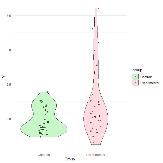
Figure 1 – Outcome distribution by group
Robust tests as back-up
If the data suggest violated assumptions, it is common to also run a robust test. Like others (Erceg-Hurn & Mirosevich, 2008; Wilcox, 2013), I argue for carrying out robust tests from the start, instead of as a backup option. Generating multiple results creates the danger of p-hacking (commonly fishing for p < α, e.g., when testing for the existence of an effect). Preregistration can and must specify how conflicting results are handled—commonly, by preferring the robust alternative over the standard test when one yields p < α and the other p ≥ α (Wagenmakers et al., 2012). In these cases, though, running only the robust test from the outset would have led to the same conclusion. The standard test is redundant. In the simulated example, the nonsignificant result (p ≥ .05) from robust linear regression contrasts with the significant result (p < .05) from OLS regression. This leads to the same conclusion as if only the robust test had been conducted. In the final chapter, I will report the results of several other, not yet fully robust alternative methods to OLS regression. Regardless of these results, if the most robust test is considered the most trustworthy, the conclusion of no evidence for an effect remains.
Another prevalent practice may subtly undermine scientific rigor: In the instance of two (or more) conflicting results, one might openly report both and interpret them together as 'unclear', ‘mixed’ or 'partial evidence', thereby implicitly treating both results as equally informative. However, because one still needs to make a binary decision (e.g., pursue further research or try an intervention assuming the tested effect exists), one may actually behave as if there were evidence. In this case, the nominal α is subtly exceeded because there were two opportunities to produce an ‘unclear’ result, which implicitly allows one to act as if the effect exists (Gelman & Loken, 2014).
Sensitivity analysis shows how sensitive a result is to choices made in the analysis and the corresponding assumptions. This enables readers to decide for themselves which assumptions and, accordingly, which results to follow (Saltelli et al., 2008). Multiverse analysis takes the radical approach of conducting all conceivable variants and informing readers transparently about all their results (Steegen et al., 2016). This seems particularly appropriate when, for example, data can be operationalized in a variety of ways. However, this could also indicate poor theoretical foundation (Scheel, 2022) or weaknesses in measurement (Anvari et al., 2025), necessitating data exploration to disclose flexibilities before confirmatory testing (Höfler et al., 2023). It has been criticized that by presenting all analyses, each is implicitly given equal weight, even though some represent ‘model specifications that are clearly inferior to alternatives’ (Auspurg, 2025). When researchers restrict the analyses to those with a plausible foundation, presenting the remaining variety of results seems reasonable, as long as we only consider the paper at hand. It becomes difficult when a binary decision must be made outside a publication and is based solely on the uncertainty in the results rather than on justifying the preference for a particular set of assumptions and the single result that follows from them.
Robust testing from the outset is epistemically well-founded
Fundamentally, empirical science should subject hypotheses to risky testing—so that if a hypothesis were false, the test would likely produce contradictory evidence. That is, tests should be severe, with large and adhered to falsification rates of 1 − α (false positives) and 1 − β (false negatives) (Mayo, 2018). However, anomalies in data—such as extreme values or outliers that disproportionately influence results—can compromise the intended error rates (in addition to other model–reality mismatch; Gigerenzer, 2004), making a false hypothesis appear corroborated or a true hypothesis appear uncorroborated (Wilcox, 2013).
Empirical testing has to be robust across random perturbations to increase reliability and protect inference from flaws in the analytical model. A test should not be passed (or unpassed) just because of faulty assumptions embedded within it (Popper, 1959). Moreover, anomalies such as extreme values and outliers are likely to occur inconsistently across studies. When analyzed, for instance, with the two independent samples t-test, one study might corroborate an effect while another might not. As Popper (1959, p. 66) stated, ‘non-reproducible single occurrences are of no significance to science.’ Such lack of replication distorts scientific communication and leads to unnecessary and misleading debates about substantive reasons for differing results, where the variation is just due to unmet assumptions in the statistical method. Robust statistical tests can mitigate these problems by reducing the influence of outliers, extreme values, Non-Normality, and heteroscedasticity (Erceg-Hurn & Mirosevich, 2008; Field & Wilcox, 2017; Rousseeuw et al., 2004; Rousseeuw & Leroy, 2005; Wilcox, 2013). If scientific reputation is to shift from publication count to replication success (Nosek et al., 2022), robust tests are preferable.
Scientific communication must be clear about the scope of the hypothesis being tested. T‑test, ANOVA, and OLS regression are routinely used to test population-average effects (though this is rarely made explicit), via mean group differences or, in the regression context, the average outcome change per unit of a predictor. Estimates of these effects (and thus the tests based on them) carry broader interpretability only when they closely reflect the true effect in many individuals. If anomalies such as extreme values or outliers dominate them, they are only applicable to a few individuals. This results in a tacit and unjustified narrowing of the inference scope (Altman & Krzywinski, 2016; Huber & Ronchetti, 2009).
Robust linear regression, the exemplary method illustrated here and alternative to OLS regression, precisely compensates for this. It weights the remaining individuals so that each contributes approximately the equal amount to the parameter estimates, in the same way as in OLS regression under its assumptions (normally distributed residuals with equal variance; Huber & Ronchetti, 2009; Wilcox, 2013). In the simulated example, two observations in the experimental group receive weights smaller than 10^-8 and are thus identified as outliers, essentially omitted from the analysis. Six further observations are down-weighted with weights in the range between 0.01 and 0.75 (rounded values). In the control group, all weights exceed 0.75. Five observations across both groups received a weight of 1.00, which means that they are fully trusted.
The final argument is an epistemic advantage of not reacting to unexpected data features. In the Popperian tradition, the substantive hypothesis should make a prediction, for example about an average effect, which may turn out to be right or wrong (Popper, 1959; Mayo, 2018). Together with a decision rule (e.g. the one-tailed p-value in the chosen statistical test must be smaller than α), it then predetermines which observations support the hypothesis and which do not. This requires fully specifying an analytical model, so that once data are collected, the test yields either p < α or p ≥ α (Lakens & DeBruine, 2021). When p < α as predicted, the test retains evidential value, simply because the prediction succeeded—even if the analytical model is imperfect and can be improved post-hoc (Box, 1976; Huber & Ronchetti, 2009; Uygun Tunç et al., 2023).
Which alternative test is appropriate?
Given the premise that a test should ideally be based on a relevant quantity and robust to Non-Normal distribution, unequal variances, and extreme values and outliers, it is important to know to which extent common alternative methods possess these properties (Kim & Li, 2023; Mair & Wilcox 2020; Potvin & Roff, 1993; Wilcox, 2013, and Wilcox & Rousselet, 2018).
The example employed robust linear regression with a dummy variable for the binary predictor, so that the estimate of the β coefficient equals the sample mean difference. This allows one to test the same as the usual Student's t-test: hypotheses on differences in means. I used the R package ROBUSTBASE (Maechler et al., 2021) for this. The most common alternative test here is the Mann-Whitney U test. It has been argued to be largely robust against Non-Normality, unequal variances, extreme values and outliers (Zimmerman, 1994). However, outliers are still included in the analysis. They count as the largest values and thus affect the result. This limitation applies to all rank-based methods, such as the Spearman rank correlation. Besides, the U test does not examine the same quantity as the standard test. Whereas the t-test is based on the difference in the mean between two populations and is therefore closer to the data, the U-test compares rank sums between groups. Although this often makes no practical difference, exceptions have been found—for example when distributions differ in spread or shape but have equal means, the U-test may signal a difference even though the means are equal in the population (Fay & Proschan, 2010; Bürkner et al., 2017). Yet, the test statistic of the U-test can be converted into a different quantity: the ‘common language effect size’ (CL), the probability that a randomly selected individual from one group will have a higher value than a randomly selected individual from the other group (McGraw & Wong, 1992). This effect size, also known as the ‘probability of superiority’, is often reported alongside ROC (Receiver Operating Characteristic) curve analysis. In R, the pROC package computes CL from the U-test statistic.
In the simulated example, the U test, calculated with the wilcox.test() function in the BASE package, yielded a test statistic of W = 318 (the rank sum in the control group) and a p-value of 0.051. The common-language effect size is estimated as 0.65, with a 95% confidence interval of 0.504 to 0.79. This result is significant because the interval does not include the null value of 0.50. The difference with the p-value from the U test arises from slightly different numerical approaches in the two computations, which would be decisive if the U test were the most robust method used here.
Unlike the U-test, the exact t-test also compares means. Its robustness comes from computing p-values via all possible data permutations rather than relying on distributional assumptions (Winkler et al., 2014). However, because (as in all permutation-based methods) extreme values and outliers reappear in many permutations, the exact t-test, is only partially robust to them. Likewise, it gives a z statistic of -2.47 and a p-value of 0.009 in the example, evaluated with the R package WRS2. Full robustness is provided by the trimmed and Winsorized versions of the t-test, also implemented in WRS2. These, similar to M-estimation in robust linear regression, downweigh extreme values and outliers according to predefined criteria. The trimmed t-test (with the default 20% trimming) gives a test statistic of t = 1.52 (df = 24.53) and a p-value of 0.141. Finally, the Winsorized t-test yields a test statistic of -0.41 (adjusted degrees of freedom) and a p-value of 0.289, thus demonstrating the desired robustness in this example.
The ROBUSTLMM package extends robust linear regression to more complex multilevel data, enabling the fitting of robust mixed-effects models and taking into account correlations between observations (Koller, 2016). Although, unlike rank and permutation-based methods (Potvin & Roff, 1993), robust linear regression models can handle control variables and interactions, even across multiple levels (Rousseeuw et al., 2004). Yet they remain limited to testing linear relationships with the outcome, perhaps after suitable data transformation.
In the frequent case of multiple measurements, when researchers use more complex, regression-based methods, they routinely employ certain robust features. These mainly involve robust estimation of standard errors, along with the confidence intervals and p-values computed from them. In particular, the resampling technique of bootstrapping and the Huber–White sandwich estimator account for Non‑Normality and heteroscedasticity and are available in software implementations across a wider range of models: not only linear models but also generalized linear models, their extensions and structural equation models (Field & Wilcox, 2017; Mansournia et al., 2021). Bootstrapping can be applied in smaller samples because it relies less on asymptotic distributional assumptions, but extremely small samples may still be problematic. Yet, both bootstrapping and the sandwich estimator do not alter the coefficient estimates, leaving them vulnerable to outliers and extreme values (King & Roberts, 2015).
In the data example, the experimental versus control group effect estimate remains 1.26 in both cases. The sandwich estimate of its standard error equals 0.49, yielding a p-value of 0.012. Likewise, bootstrapping produces a false positive result: the bootstrapped standard error equals 0.50, giving a p-value of 0.010 (computed from the bias-corrected and accelerated confidence interval with 5000 resampling replications).
Another class of models worth mentioning is generalized additive models (GAMs). They handle Non‑Normal outcomes similarly to generalized linear models, but estimate linear effects such as mean differences or slopes (Aeberhard et al., 2021). The R package MGCV offers robust standard errors, obtainable through sandwich estimators, as well as more detailed variance modeling (Wood, 2025). Combinations with M‑estimated coefficients have been proposed but are not yet widely established beyond expert use (Aeberhard et al., 2021). A final, broadly applicable option is to fit a possibly non-linear model and then — in a post hoc step — compute and test linear contrasts using the R package MARGINALEFFECTS (Arel-Bundock et al., 2024). This includes generalized linear models, mixed effects models, GAMs and Bayesian models (see below), but can not be combined with M-estimation.
R packages for robust methods have been reviewed in more detail by Todorov (2024).
Bayesian approaches
The discussion so far has been limited to frequentist tests, which require the error rates α and β to be fixed before any data inspection. This conception does not carry over to Bayesian testing approaches such as Bayes factors, where each new observation updates the evidence for the competing hypotheses. Because Bayes factors accumulate evidence sequentially, their outcomes can depend on the order in which data arrive and on whether data collection is stopped early (for example, when the Bayes factor exceeds a threshold such as > 10 or < 1/10). Some decision-theoretic Bayesian approaches avoid these dependencies by basing decisions solely on the final posterior distribution and disallowing early stopping of data collection (Berger, 1985; Robert, 2007). Schnuerch et al. (2024) have recently proposed a procedure, with an accompanying web application, that controls the error rates for a Bayesian variant of the t-test.
Robust Bayesian tests are possible without predefined α and β values, though the topic is technically complex, still developing, and not yet widely applied. Standard ‘default’ priors (typically Normal) combined with a Normal likelihood—as in Bayesian linear regression, t-tests, or ANOVAs—are not inherently robust to outliers, extreme values, heavy tails, or heteroskedasticity. Robustness however improves substantially when the Normal likelihood is replaced with a heavier-tailed t-distribution or a Contaminated-Normal (mixture) model, which assumes the data are a mixture of a target Normal distribution and an outlier distribution. Nonparametric approaches, such as the Bayesian bootstrap, can also provide some protection, though their effectiveness depends strongly on the model structure and the choice of priors (Kennedy et al., 2017; Wilcox, 2013).
Finally, jointly predefining α and β while achieving full robustness appears theoretically possible in Bayesian testing, but it is not yet implemented in established, CRAN‑quality R packages.
Discussion
Time has come to overcome standard statistical tests whenever their assumptions are unlikely to be fulfilled. This would reduce unnecessary variation in results both within and between studies. Within studies, the flexibility in dealing with the variation must be rigorously disclosed to ensure rigorous testing, which can otherwise be subtly undermined. Between studies, the common usage of robust methods shall reduce the number of non-replicated findings, facilitating scientific communication in a field that is already burdened by otherwise occurring variance between study results (Nosek et al., 2022).
Yet some costs of using robust methods need to be mentioned. First, on a technical level, instances have been described in which they do not perform as well as desired. Robust standard errors and thus p-values may be unnecessarily high when a model is correctly specified (King & Roberts, 2015). Examples for the opposite, somewhat deflated p-values, have also been found, especially in small samples (Mansournia et al., 2021). Robust linear regression is based on weights derived from the data, and the standard errors of the estimated coefficients do not account for the randomness in these weights. This can sometimes produce inaccurate results, especially in small samples (Rousseeuw & Leroy, 2005; Mair & Wilcox, 2020). On the interpretational level, robust standard errors and regression coefficient estimates do not correct for model misspecification. In fact, they can create a false confidence in a result, distracting from flaws in design and analysis (King & Roberts, 2015). Nevertheless, the benefits of robust tests outlined in this paper should outweigh these limitations by far.
To make robust testing more commonplace, training students and young scientists seems to be a promising lever. Early-career researchers do not have to defend many publications based on conventional tests. Teaching should refer to the replication crisis and appeal to the advantages of more reliable and sustainable scientific results. At the same time, the toolbox of robust alternatives should be extended further toward full robustness, also in non-linear and Bayesian models against all foreseeable data issues and, in that vein, their robustness properties should be better understood. Ultimately, the methods should be implemented and explained in a way that facilitates access and application.
Acknowledgements
Preprint version 4 of this article has been peer-reviewed and recommended by Peer Community In Psychology (https://doi.org/10.24072/pci.psych.100025; Nettle, 2025)
Funding
No funding was received to assist with the preparation of this manuscript.
Conflict of interest disclosure
The author declares that he complies with the PCI rule of having no financial conflicts of interest in relation to the content of the article, and has no non-financial conflicts of interest.
Data, scripts, code, and supplementary information availability
Script and code are available online (https://doi.org/10.17605/OSF.IO/FW695; Höfler, 2025). Simulated data can be reproduced through the provided code.