
 CC-BY 4.0
Introduction
A fundamental aspect of ecology is identifying and characterizing population processes. A common definition of a population is “a group of organisms of the same species occupying a particular space at a particular time that are capable of interbreeding” (Krebs, 1994; Williams et al., 2002); hereafter, we refer to a biological population using this definition. Because a complete census is rare, we almost always rely on sampling to make inference about a biological population, and the scope and strength of inference depends on our ability to sample the population appropriately. For mobile species, this crucial task can be challenging. One of the important characteristics of population sampling is the portion of the population present at the time and place of sampling; hereafter, we refer to the part of the biological population at risk of sampling as the statistical population.
The conceptual distinction between a biological population and a statistical population has been around for decades, though the terminology has varied considerably (Waples & Gaggiotti, 2006). In addition to biological and statistical (Krebs, 1999), notable examples include target and sampled (Cochran, 1977), natural and local (Andrewartha & Birch, 1954), and resource and statistical (Reynolds, 2012). Regardless of the terminology, the distinguishing principle is the same: one population is what we really want to know something about (biological) and the other is what we use to infer what we want to know (statistical). In practice, it is important to remember that sampling-based inference directly applies only to the statistical population; logic, assumption, or additional information are needed to extend inference to the biological population.
When the biological and statistical populations are identical, direct statistical inference applies to both populations. However, when the proportion of the population at risk of sampling is <1, then the statistical population is usually a subset of the biological population (Figure 1); we refer to this situation as population misalignment. Population misalignment also has been called a frame error (Reynolds, 2012), drawing from the fact that the sampling frame defines the proportion of the biological population at risk of being sampled (i.e., the statistical population).
Population misalignment can occur for a variety of reasons. Common reasons include those that are physical (e.g., natural barriers), logistical (e.g., cost, safety), legal (e.g., landownership boundaries), political (e.g., international borders), and even biological (e.g., non-breeding). For example, the Pacific walrus (Odobenus rosmarus divergens) population ranges across marine waters of Alaska and Russia, though sampling rarely covers the entire region mostly owing to complications with securing the necessary international permits (e.g., Beatty et al., 2022). Consequently, assuming individuals can move freely, they may not be exposed to sampling consistently, which potentially affects inference about the biological population.
Analytically, we often view population misalignment as a form of temporary emigration, whereby individuals are temporarily not exposed to sampling (Kendall et al., 1997). Temporary emigration is an oddly vague process with biological and statistical drivers that usually are confounded. For example, individuals may temporarily emigrate for biological reasons like searching for food or avoiding predation, statistical reasons such as unequal sampling probability owing to a small or varying frame, or a combination of both. Ultimately, temporary emigration is a detection issue. If it occurs randomly with all animals equally likely to be part of the statistical population across sampling occasions, temporary emigration will cause large residual variance and reduced precision of abundance estimates; if it occurs non-randomly, e.g., with a temporal trend, it will bias estimates.
Over the last few decades, many analytical approaches have been developed to account for temporary emigration when estimating abundance. The most notable methods are capture-recapture models that use robust design (Kendall et al., 1997) or are spatially explicit (Royle & Young, 2008), extensions of N-mixture models (e.g., Chandler et al., 2011), thinned point process models (e.g., Mizel et al., 2018), and models that combine methodology (e.g., Powell et al., 2000; Amundson et al., 2014). These approaches use spatial and temporal replicates with short periods of closure (i.e., no movement into or out of the statistical population; hereafter replicate sampling) or the ability to identify individuals during sampling (hereafter repeat sampling) to estimate temporary emigration and abundance of the biological population, which is sometimes referred to in this context as the superpopulation (Schwarz & Arnason, 1996). While these models are flexible and powerful, they require data from replicate and repeat sampling, which is not feasible for all species and habitats.
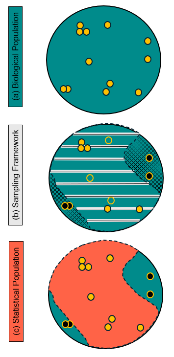
Figure 1 - Schematic illustrating the relationship between the (a) biological population, or the population of interest; (b) sampling framework with line transects (black lines with gray rectangles) along which individuals are sampled (solid yellow circles) or not sampled (open yellow circles) and inaccessible areas (cross-hatching) that contain a portion of the biological population (solid black circles); and (c) statistical population, which is defined by the extent of the sampling frame in (b).
An alternative approach to handling a population misalignment that does not require replicate or repeat sampling is to decompose the detection process. Nichols et al. (2009) described four components of overall detection (p): (1) ps, the probability that the individual’s home range includes at least a portion of the sample area; (2) pp, the probability of presence within the sample area during a survey; (3) pa, the probability of availability given presence; and (4) pd, the probability of detection given presence and availability. The first component (ps) simply confirms that an individual is a member of the biological population, and the last component (pd) refers to the actual observation process, that is whether an individual was observed. Jointly, the second and third components (pp and pa, respectively) describe temporary emigration, with the second component (pp) being spatial temporary emigration, and the third component (pa) as random temporary emigration (Kery & Royle, 2016). A major advantage to using this approach is that each component can be estimated separately using different datasets and even different data types (Hostetter et al., 2019), making it suitable for all species and habitats provided that data for estimating components are available.
We applied this approach to account for population misalignment of the Kittlitz’s murrelet (Brachyramphus brevirostris), a highly mobile, non-territorial, ice-associated seabird that is irregularly distributed across coastal Alaska and eastern Russia. Several aspects of this species’ life history complicate methods that rely on replicate or repeat sampling to estimate spatial temporary emigration. Unlike most seabirds, Kittlitz’s murrelets do not nest in colonies, but instead nest solitarily at low densities, usually in remote inaccessible locations (Kissling et al., 2015a). Thus, populations cannot be monitored at colonies like most seabirds where replicate and repeat sampling is practical and efficient. Additionally, owing to the small size, cryptic behavior, and low and variable breeding propensity in this species, capture-recapture and resight models are not reasonable options. It is nearly impossible to resight banded or marked murrelets on the water or in flight and recapture rates are too low to be useful for estimating abundance (Kissling et al., 2015b).
Instead, the only viable way to monitor Kittlitz’s murrelet populations is with boat-based abundance surveys that are conducted during the breeding season when most murrelets concentrate in bays and fjords often near tidewater glaciers (Day et al., 2020). A design challenge and safety concern for these surveys is the presence of icefloes, large tidal fluctuations, glacial river debris, and the possibility of rough seas. These dynamic conditions can restrict boat access to portions of the study area and cause murrelets to redistribute over short time intervals, resulting in time-varying statistical populations and a population misalignment that cannot be handled with replicate sampling, as neither the murrelets nor the habitat can meet the closure assumption.
We developed a hierarchical Bayesian modeling framework to estimate abundance of a biological population of the Kittlitz’s murrelet in a dynamic environment. Our framework utilizes datasets from telemetry flights to locate radio-tagged murrelets, boat-based distance sampling surveys, and dive behavior trials to account for all components of detection probability (ps, pp, pa, pd). Our primary objective was to develop an analytical tool to account for misalignment of the statistical and biological populations of this unusual species so that we could generate unbiased abundance estimates for further use in an integrated population model (Kissling et al., In revision). More specifically, here, we aimed to (1) estimate detection probability components and their variation across space and time; (2) investigate predictability of pp using environmental covariates; and (3) estimate abundance and trend of the statistical (without pp) and biological populations (with pp) and identify any sources of bias. We also wanted to assess whether we delineated the biological population of Kittlitz’s murrelets in our study area appropriately.
Material and methods
Study area
Our study was centered in Icy Bay, Alaska, USA, located in the northeastern Gulf of Alaska and ~110 kilometers northwest of the town of Yakutat (Figure 2). Icy Bay is a highly dynamic glacial fjord system that has experienced multiple, rapid ice advances and subsequent retreats over the past ~3,800 years with the most recent retreat of approximately 40 km during the 20th century (Barclay et al., 2006).
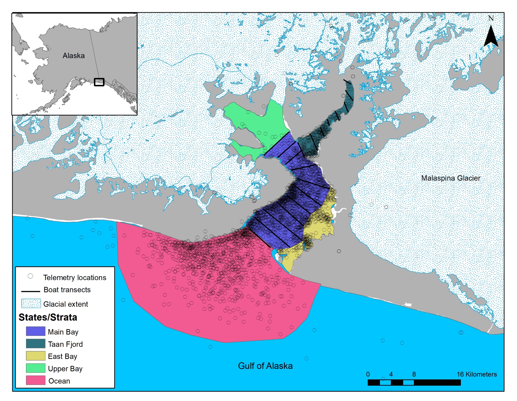
Figure 2 - Map of study area, Icy Bay, Alaska, where we conducted boat and telemetry surveys to estimate abundance of Kittlitz’s murrelets. Our sampling area during telemetry flights comprised five spatial states that collectively formed the extent of the biological population: Icy Bay (Main Bay and Taan Fjord sub-states combined), East Bay, Upper Bay, Ocean, and nest. During boat surveys, only the Icy Bay state, with Main Bay and Taan Fjord as strata, was regularly accessible and formed the extent of the statistical population. The gray-shaded area is land.
Currently, Icy Bay comprises a shallow outer bay and a deeper inner bay. The outer bay is adjacent to the Gulf of Alaska and measures 6 km wide at the mouth. The inner bay is divided into four distinct fjords with each terminating at an active tidewater glacier. Of these fjords, only Taan Fjord is regularly accessible by boat (Figure 2) The Malaspina Glacier, the largest piedmont glacier in North America, is situated to the east and empties meltwater and glacial sediment into Icy Bay via the Caetani River system, which can restrict boat access to the eastern side of the bay. During periods of high river flow, debris and sedimentation settle near the outflow and the marine waters become too shallow to navigate a boat safely. In addition, two small bays (Riou and Moraine bays) are located on the eastern side of Icy Bay and they have submerged marine sills at their mouths making it difficult to access them during low tides. The total surface of Icy Bay is approximately 263 km2, but typically the upper half of the bay is covered in thick ice floes and large icebergs, resulting in an open water surface area of ~160 km2 with considerable variability within and across years depending on glacial calving activity.
Data collection
Boat surveys
From 2005 to 2017, we conducted two boat-based abundance surveys between 1 and 15 July in each of eight years (2005, 2007–2008, 2010–2012, 2016–2017); in 2009, we conducted only one survey on 17 July because of logistical constraints. The target sampling area was ~160 km2 and contained 19 line transects total, with 11 transects in the Main Bay and 8 transects in Taan Fjord (Figure 2), though actual sampling effort varied for each survey because of access issues (Table 1). Generally, we completed surveys in a single day, though rarely it took two days, depending on tides and other logistical factors. Boat surveys involved line transect distance sampling, following the protocol described in Kissling et al. (2007, 2011), with one exception; in 2016 and 2017, we estimated the angle and distance from the boat to each murrelet group as opposed to estimating perpendicular distance from the line transect (all other years). We also recorded group size, behavior (water, flying), and foraging activity of all Brachyramphus murrelets observed. Both Kittlitz’s and its congeneric marbled murrelet (B. marmoratus) occur in Icy Bay and can be difficult to distinguish, especially at a distance; if an observer was unable to identify a murrelet (or group of murrelets) to species, it was recorded as an unidentified murrelet(s).
Table 1 - Sample sizes and effort by survey type for estimating abundance of a biological population of Kittlitz’s murrelets, Icy Bay, Alaska, 1–15 July 2005–2017. Truncation distance was used to model the detection function to estimate probability of detection (pd) with distance sampling data.
Year | Boat surveys | Telemetry surveys | |||||
|---|---|---|---|---|---|---|---|
# surveys | Portion of sampling area surveyed | Truncation distance (m) | 15-day period | ||||
Survey 1 | Survey 2 | # flights | # radio-tagged individuals | # locations | |||
2005 | 2 | 0.85 | 0.85 | 250 | - | - | - |
2007 | 2 | 0.75 | 0.74 | 281 | 4 | 24 | 82 |
2008 | 2 | 0.75 | 0.70 | 278 | 8 | 20 | 137 |
2009a | 1 | 0.91 | - | 288 | 5 | 20 | 85 |
2010 | 2 | 0.67 | 0.91 | 242 | 3 | 24 | 58 |
2011 | 2 | 0.77 | 0.73 | 210 | 4 | 27 | 100 |
2012 | 2 | 0.75 | 0.56 | 181 | 4 | 17 | 54 |
2016 | 2 | 0.91 | 1.00 | 325 | - | - | - |
2017 | 2 | 0.91 | 0.90 | 323 | - | - | - |
aBoat survey conducted on 17 July 2009; telemetry survey information presented here for 1–15 July 2009.
Telemetry surveys
We captured Kittlitz’s Murrelets on the water using the night-lighting method (Whitworth et al., 1997) in the Icy Bay study area between 8 May and 3 June, 2007–2012 (Figure 2; see Kissling et al., 2015a, 2015b, 2016 for details on capture, handling, tagging, and relocating). Following capture, we transported murrelets to a larger vessel for processing, which included morphometric measurements, blood sampling for sex identification, and banding. We deployed very-high-frequency (VHF) radio transmitters on a subset of after-second-year murrelets captured each year. We attached the transmitters (Advanced Telemetry Systems, Inc., Isanti, Minnesota; model number A4360; 110-day battery life) using a subcutaneous anchor on the bird’s back between the scapulars (Newman et al., 1999). If both birds of a pair were captured, we randomly selected one bird to radio-tag to ensure independence. We released murrelets immediately after processing was complete.
We attempted to locate radio-tagged murrelets 2–5 times per week for at least eight weeks after tagging using fixed-wing aircraft equipped with “H-style” antennas mounted on the struts. We were not able to search for tagged birds using a strict design, but instead aimed for complete coverage of the study area, as shown in Figure 2, in a systematic way that allowed for safe flying. We first attempted to locate all murrelets on the water in the Icy Bay study area within gliding distance of shore; if murrelets were not detected at sea, we flew over all assumed potential nesting habitat within reason (e.g., fuel constraints) to locate incubating birds. We conducted telemetry flights on the same day as boat surveys; on occasion, we had to fly the telemetry survey on the following day because of aircraft availability. All telemetry flights were completed in less than four hours.
During each flight, we mapped ice conditions into five categories of increasing ice density: none, brash ice, open pack ice, close pack ice, and very close pack ice. We defined brash ice as accumulations of floating ice made up of fragments not more than 2 m across, open pack ice as low concentration pack ice with many leads and polynyas and the floes generally were not in contact, close pack ice as moderate concentration pack ice with the floes generally in contact, and very close pack ice as high concentration pack ice with very little water visible (Bowditch classification; NOAA, 2007). Following each flight, we digitized these maps in ArcGIS (ESRI, v10.7.1) and estimated ice cover (km2) by category in the study area on that day. We then assigned all locations of radio-tagged murrelets to an ice category using the ice condition maps for each corresponding telemetry flight.
Environmental data
We compiled environmental data for murrelets located during telemetry flights. Using the date and time of each location, we determined tide direction, which represented the vertical movement of water, as ebb or flood, and tidal current strength, the horizontal movement of water, following Kissling et al. (2007). We also acquired the daily precipitation (mm), which affected freshwater input volume and turbidity, and average daily wind speed (m/sec), which influenced icefloe movement and ocean surface conditions, from a weather station in Icy Bay (https://www.ncdc.noaa.gov/cdo-web/). Lastly, we calculated the proportion of the Icy Bay state (i.e., the area sampled during boat surveys) that was covered in ice (all categories) on the flight day. See ‘Predicting probability of presence’ below for hypotheses regarding these environmental data.
Data analysis
Components of detection probability
We considered detection probability components individually, which allowed for use of different datasets, and then combined those necessary in a joint likelihood model to estimate abundance (see below; Figure 3). This approach was efficient, as two components of detection probability, ps and pa, were deemed to be close to 1 and unnecessary in the abundance model.
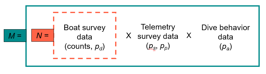
Figure 3 - Schematic showing data sources for estimating abundance of the statistical population (N) and the biological population (M) of Kittlitz’s murrelets in Icy Bay, Alaska, 2005–2007, with the four components of detection probability, where ps is the probability that an individual’s home range includes at least a portion of the sample area, pp is the probability of presence within the sample area during a boat survey, pa is the probability of availability during a boat survey, and pd is the probability of detection by an observer during a boat survey. For this study, we assumed ps and pa were 1 based on previous work described by Kissling et al. 2024b and Lukacs et al. 2010, respectively.
We determined that ps, the probability that an individual could be included in the sampled area during a boat survey, was 1 in all years by examining both home ranges (95% utilization distribution [UD]) and core use areas (50% UD) of radio-tagged murrelets (Kissling et al., 2024b). The UDs for all individuals intersected with the sampled area during boat surveys in all years. Therefore, we did not include ps in our model.
We estimated pp, the probability that an individual was present in the sampled area during a boat survey, using location data from radio-tagged murrelets. Following Kissling et al. (2015b), we assigned each telemetry location to one of five spatial states (Figure 2): Icy Bay, which comprised Main Bay and Taan Fjord sub-states and was the core area sampled by boat; East Bay, which was too shallow for a boat; Upper Bay, which was too icy; Ocean, which was too rough; or at a nest. The outer limit of the Ocean state was constrained to aircraft gliding distance to shore, and it was same area used for a multi-state survival analysis (Kissling et al., 2015b). Any telemetry locations outside of these five states were removed from our analysis (<2% of all locations); notably, none of these individuals were located again. We then merged data on spatial state and ice category for each telemetry location. We considered a radio-tagged murrelet to be present in the sampled area if it was in Icy Bay state and in ice categories of none, brash ice, or open pack ice, where we could conduct boat surveys safely. If a radio-tagged murrelet was at a nest or in the East Bay, Upper Bay, Ocean, or in close pack ice or very close pack ice, it was deemed not present.
Then, we filtered telemetry data to include locations from 1 to 15 July to overlap with our boat survey protocol. We explored the use of telemetry locations acquired in 1-, 3-, 5-, and 7-day windows surrounding the boat survey; for example, if a boat survey was conducted on 8 July, the 3-day window was 7–9 July and the 5-day window was 6–10 July. All telemetry locations collected during a specific window were used to estimate a single value of pp. In 2009, we conducted a single boat survey late (17 July) because of boat availability and poor weather and therefore, we shifted the windows to center on the later date. In all years, we found that pp varied little with window length, though precision improved (Appendix 1), which was unsurprising given that sample size increased (i.e., number of telemetry locations). Here, we report results for the 3-day window only because it was the best tradeoff between improved precision while maintaining a short temporal window around each survey. For comparison, we also report pp for the entire 15-day period (1–15 July).
We conducted boat-based dive behavior trials to estimate pa, the probability that a murrelet was available for detection (i.e., not underwater) given presence (Lukacs et al., 2010). These experimental trials consisted of approaching groups of murrelets in a boat and recording the characteristics of their response (e.g., flight or dive, distance, dive time, number of dives). We determined that the probability of a murrelet being unavailable for detection was quite low (0.032 ± 0.007; see details in Lukacs et al., 2010). Therefore, we assumed pa was close enough to 1 not to affect abundance estimates, and, like ps, did not include it in our model.
Finally, we estimated pd, or the probability of being detected given presence and availability on boat surveys, using conventional distance sampling (Buckland et al., 2001). We filtered data to include murrelets observed on the water only, i.e., we excluded flying birds from our analysis. We pooled data across both surveys each year (except 2009) and all Brachyramphus murrelets to estimate pd because observers rarely changed, and we did not expect detection probability to be different by species. We then truncated 5% of the data from the right-hand tail of the detection function (Buckland et al., 2001). We examined the effect of group size on the scale parameter of the half normal detection function, but it had no effect in any year (based on ΔAIC values and Cramer-von Mises tests) and therefore, we did not include group size in our analyses.
Then, to allocate murrelets not identified to species (i.e., unidentified Brachyramphus murrelets) during boat surveys, we estimated the probability of being a Kittlitz’s murrelet (pk), as opposed to a marbled murrelet, in two strata (m) in Icy Bay for each year (Figure 2). While Kittlitz’s murrelets are uniformly distributed throughout the bay, marbled murrelets are not; they are rarely located in Taan Fjord (Kissling et al. 2007, 2011). Therefore, we divided our sampling area into two strata, Main Bay and Taan Fjord, to satisfy the assumption of uniform distribution when estimating pk. Note that these strata were the same as the Main Bay and Taan Fjord sub-states described for pp, though they were not indexed for pp; we used different terminology to avoid confusion in the code.
Model for biological population abundance
We developed a hierarchical Bayesian modeling framework to estimate annual abundance of the biological population. Our framework combines multiple datasets in a unified analytical framework (Figure 3), and therefore, it fully accounts for uncertainty and error in parameter estimates, similar to an integrated model though without a shared parameter across all datasets (Zipkin et al., 2021). We used data augmentation to represent a relatively large number of potential but unobserved groups in our sampling area during each boat survey (Royle & Dorazio, 2008). To estimate a single value for annual abundance, we used the following joint likelihood:
\(L\left\lbrack M \right.\ \left| \left. \ data \right\rbrack = \left\lbrack L\left\lbrack \left. \ M \right|N_{i},p_{p,i} \right\rbrack \right\rbrack\ \left\lbrack L\left( p_{p,i}\left| y_{p_{p,i}} \right.\ \right) \right\rbrack\ \left\lbrack L\left( p_{d,.}\left| y_{p_{d,.}} \right.\ \right) \right\rbrack\ \left\lbrack L\left( p_{k,.m}\left| y_{p_{k,.m}} \right.\ \right) \right\rbrack \right.\ \)
where M is the abundance of the biological population; Ni is the statistical population abundance estimated for survey I; pp,i is the probability of presence for survey i; \(y_{p_{p,i}}\) is the telemetry survey data used to estimate pp,i; pd,. is the probability of detection across both surveys; \(y_{p_{d,.}}\) is the boat survey data to estimate pd,.; pk,.m is the probability of being a Kittlitz’s murrelet across both surveys by stratum m; \(y_{p_{k,.m}}\) is the boat survey data used to estimate pk,.m; and data refers to the collective boat and telemetry survey data. We estimated annual abundance of the statistical population using equation 1 without the pp,i likelihood component, which essentially assumes pp,i was 1.
We modeled pp,i on the logit scale using telemetry survey data as logit(pp,ij) = βi, where βi is the logit(pp,i.) and therefore,
\(y_{p_{p,ij}}\) ~ Bernoulli(pp,ij)
where individual locations (j) during each survey (i) were used to estimate pp,ij. We did not include covariates in this sub-model because we did not identify any that helped explain variation in pp,ij (see ‘Predicting probability of presence’ below).
We modeled pd,. on the log scale using the boat survey data with perpendicular distance of each group q from the transect line (xiq) and the half-normal detection function:
\(p_{d,.q} = \exp\left( - \frac{x_{iq}^{2}}{2\sigma_{iq}^{2}} \right)\)
where σq is the scale parameter. As noted above, we did not include group size as a covariate on σq because it did not help explain variation in pd,.. We estimated the probability of being a Kittlitz’s murrelet using the boat survey data as
\(y_{p_{k,.m}}\) ~ Bernoulli(pk,.m),
where identified groups in each stratum across all surveys were used to estimate pk,.m. We modeled group size of the augmented groups as
yg,.q ~ Poisson(λg),
where yg,.q is the observed group size q across all boat surveys and λg is mean group size.
We ran our model (equation 1) with its components (equations 2–5) by year because of long run-times (~10–12 hours) and to accommodate slight differences in data management and storage each year. Moreover, no parameters were shared across years and therefore, we would not have gained anything by running the model with all years simultaneously.
Predicting probability of presence
We attempted to predict pp of radio-tagged murrelets in the sampling area using environmental covariates with the same model described above (equation 2). The purpose of this analysis was to determine if we could estimate pp in years for which we lacked telemetry data (i.e. 2005, 2016, and 2017) and potentially improve our boat survey protocol to minimize variation in pp in the future. We considered five covariates: tide direction, tidal current strength, daily precipitation, daily average wind speed, and the proportion of Icy Bay state covered in ice. We hypothesized that pp would be higher during the flood (incoming tide) than the ebb and positively associated with tidal current strength, reasoning that these conditions would concentrate murrelet prey. We posited that pp would be negatively associated with daily precipitation because of increased freshwater input into Icy Bay, possibly reducing prey or access to prey because of higher turbidity, and positively related to daily average wind speed, as an indicator of offshore storms. Lastly, we hypothesized that pp would be inversely related to the proportion of ice in the Icy Bay state, as ice would displace murrelets.
We used a generalized linear mixed model (binomial error, logit link) with random effects for year and individual to explore our ability to predict pp with environmental covariates. We filtered telemetry data to include the same dates as our boat survey protocol (1–15 July); we also excluded murrelet locations at a nest because environmental data for those records were not relevant. We scaled all covariates to have a mean of 0 and standard deviation of 1. To assess our model, we used cross-validation by randomly selecting 80% of the records to estimate pp, then using the estimated pp to predict presence for the remaining 20%, setting a threshold of 0.5 to denote whether a murrelet was predicted to be present or not in the sampling area (e.g., Boyce et al., 2002). We then created a confusion matrix comparing predicted and actual presence to evaluate our ability to predict presence.
We ran this analysis separately from estimation of abundance for the statistical and biological populations. Our reasoning for doing so was to manage model runtime.
Estimating trend in abundance
We used a state space model to estimate trend in abundance, or the instantaneous growth rate (r), of the statistical and biological populations (i.e. without and with pp, respectively). Our state space model included a random effect for year and weighted the response variable (log abundance) by the inverse of its variance. For years with direct estimates of pp (2007–2012), we used abundance of the biological population estimated incorporating telemetry data (3-day window). In years without telemetry data (2005, 2016–2017), we used mean pp from across the 15-day period in all years, with year and individual included as random effects in the estimation process. We intended to predict pp for use in these non-telemetry years, but because our predictive power was low, we opted to use mean pp. To assess the effect of including pp in our trend estimate, we examined the root-mean-square-error (RMSE) of mean r and percent change of coefficients of variation (CV) of the geometric growth rate, lambda (λ), converted from mean r to avoid division by 0, between models without and with pp. We report trend results across all years (2005–2017).
Because we estimated abundance for each year using separate model runs, we had to run the state space model separately too. To do so, we saved the output of each model for annual abundance and used the means and standard deviations as data input for the state space model. This approach could be heuristically viewed as using informative priors, but it was a practical choice to minimize model runtime of the annual estimates.
We fit all models using JAGS (Plummer, 2003) with R 4.2.1 (R Core Team, 2019) using R2jags as an interface (Kissling et al., 2024a). We used weakly informative priors on all parameters and 3 chains of 50,000 iterations, discarding the first 15,000 per chain as burn-in. We assessed model convergence through visual inspection of trace plots and the Gelman-Rubin diagnostic (Brooks & Gelman, 1998). We assumed convergence had occurred when chains overlapped substantially, and the Gelman-Rubin diagnostic was <1.1 for all parameters.
Results
Components of detection probability
We radio-tagged 191 Kittlitz’s murrelets between 12 May and 3 June, 2007–2012. Of these, 132 birds remained alive in the study area until at least 1 July when boat surveys commenced, contributing to 516 telemetry locations that were used to estimate pp (Table 1). Across all flights and years, relocations of most radio-tagged murrelets were in the Icy Bay state (53%) where boat surveys occurred, followed by the inaccessible states of Ocean (24%), East Bay (18%), Nest (4%), and Upper Bay (<1%; Appendix 2a). Only 5% of murrelets in the Icy Bay state were in close pack ice; the remainder were in open pack ice (8%), brash ice (15%), or no ice (72%; Appendix 2b).
Across all years, the median of pp was 0.50 (standard deviation [SD]=0.02). During the 15-day period in which boat surveys were conducted, median annual estimates of pp ranged from 0.35 (SD=0.06) to 0.65 (SD=0.04; Figure 4a), which was similar to median estimates from the 3-day window surrounding each survey (0.32 [SD=0.10]–0.76 [SD=0.09]; Appendix 1). Within a year, pp varied little, as indicated by the points falling close to the identity line (Figure 5). Although the 95% credible intervals (CrI) across surveys and within a year always overlapped, they narrowed as the window widened, reflecting an increase in the number of telemetry locations used to estimate pp (Appendix 1).
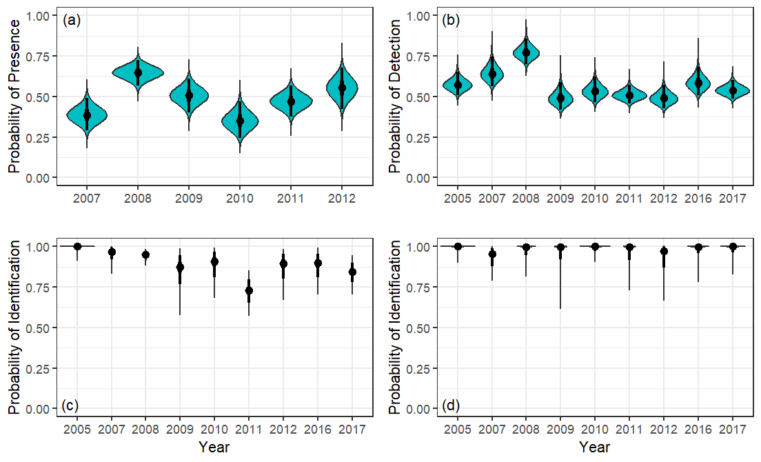
Figure 4 - Posterior distributions (teal) of estimates of detection probability components for Kittlitz’s murrelets, Icy Bay, Alaska, 2005–2017. Components are (a) probability of presence (pp), (b) probability of detection (pd), and probability of being a Kittlitz’s murrelet (pk) in (c) Main Bay and (d) Taan Fjord strata. The median of the estimate is denoted with a point, the 50% credible interval with a thick line, and the 95% credible interval with a thin line. Note that for pd (b), truncation distance varied across years (Table 1).
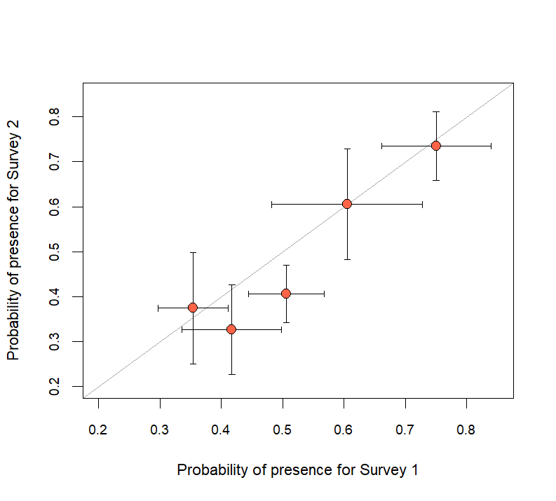
Figure 5 - Probability of presence (pp) for the 3-day window by boat survey within a year. The error bars describe the standard deviations of the estimate and correspond with the respective axes. The identity, or 1:1 line, is included in gray.
Our ability to predict pp using five environmental covariates was generally poor (Figure 6). We correctly predicted 62% of the observed outcomes and incorrectly predicted 38%. Of the environmental covariates examined, proportion of Icy Bay state covered in ice was the only one with 95% CrI that did not include 0 (βice = -0.356, CrI = -0.665, -0.059). While our hypothesis that pp would be higher during a flood tide was not supported (βtide = -0.006, CrI = -0.345, 0.356), we found that pp was more variable with a flood compared to an ebb tide (Figure 6b).
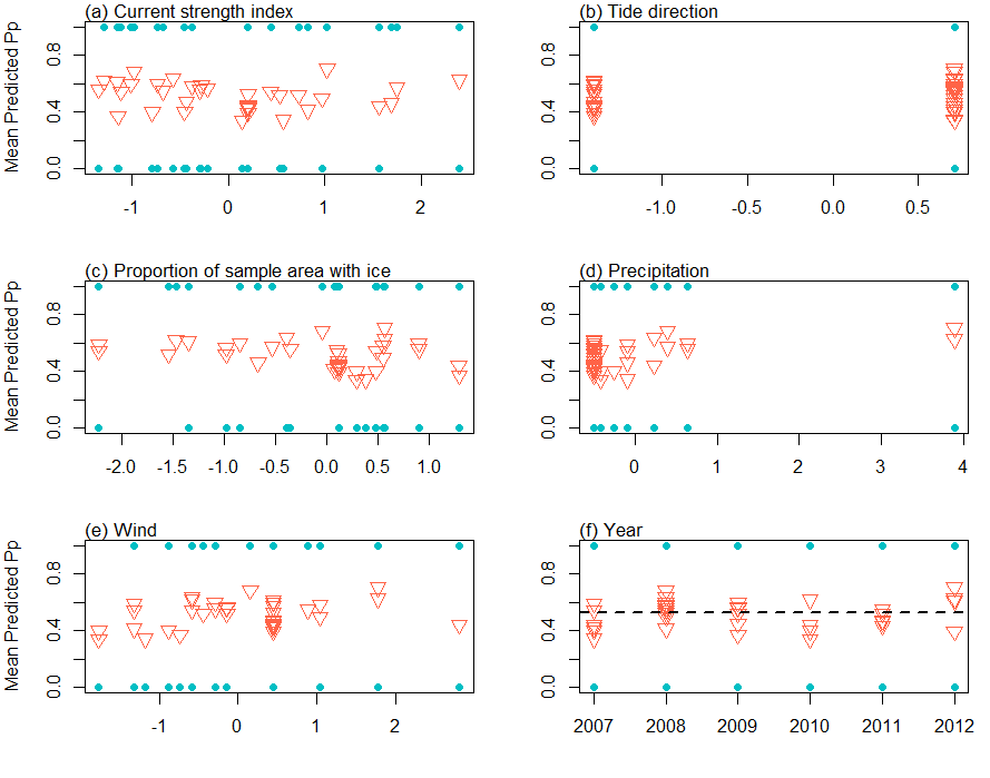
Figure 6 - Distribution of observed outcomes (teal points) and predicted probability of presence (pp; orange triangles) using environmental covariates for Kittlitz’s murrelets, Icy Bay Alaska, 2007– 2012. Covariates on x-axis are scaled; see ‘Methods’ text for description. For year (f), the dotted line denotes the mean pp across all years in the observed dataset.
Between 2005 and 2017, we conducted 17 boat surveys for Brachyramphus murrelets, of which only one covered the sampling area completely (mean fraction of sampling area covered=0.80, range=0.56–1.00; Table 1). This limitation of boat survey coverage due to shifting ice underscores the dynamic nature of our study area. Median annual estimates of pd varied from 0.49 to 0.77 with CVs below 9% (Figure 4b). The probability that a detected Brachyramphus murrelet was a Kittlitz’s murrelet, not a marbled murrelet, was high in both spatial strata, but lower and more variable in the Main Bay (range=0.72–1.00) compared to Taan Fjord (range=0.95–1.00; Figure 4c,d).
Abundance and trend
Abundance estimates of the statistical population were positively correlated with estimates of pp; that is, when pp was low, abundance was low, and vice versa (Figure 7). In all years, biological population abundance estimates were generally stable across all window lengths (Appendix 3). In years when two boat surveys were conducted, our model with pp reduced CVs of annual abundance estimates by 13–35%; in the year with only one boat survey (2009), CVs increased by 270% (Figure 8), likely because the CV of the 2009 population estimate was highly underestimated.
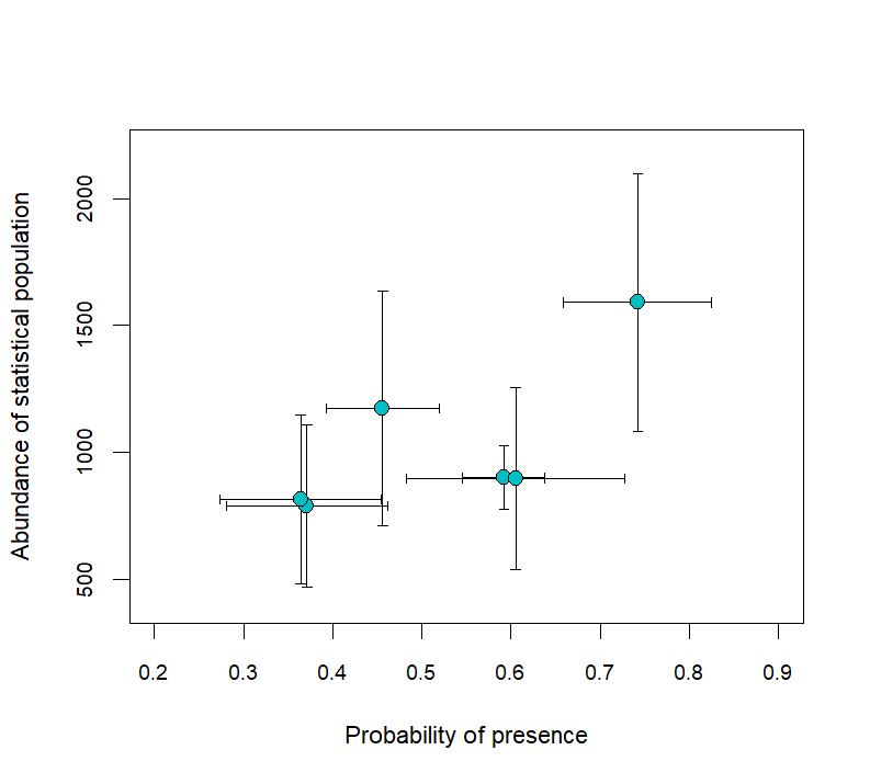
Figure 7 - Probability of presence (pp) across both surveys for the 3-day window by abundance of the statistical population, i.e., without pp. The error bars describe the standard deviations of the estimate and correspond with the axes.
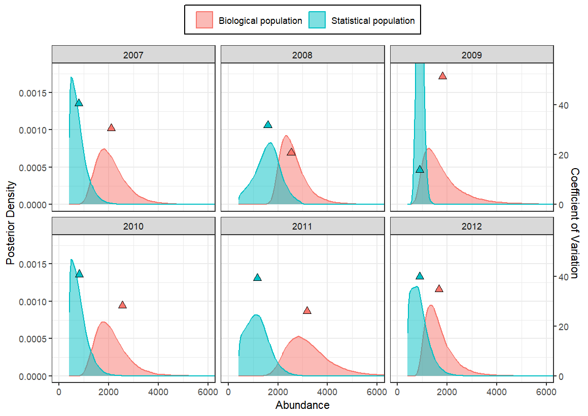
Figure 8 - Posterior distributions of annual abundances estimate for the Kittlitz’s murrelet and corresponding coefficients of variation (triangles) without probability of presence (pp; statistical population) and with pp (3-day window; biological population) around corresponding boat surveys, Icy Bay, Alaska. In 2009, when only one boat survey was completed, the posterior distribution was extremely narrow (overly precise) and extends beyond the y-axis limits of this figure for display purposes.
From 2005 to 2017, the trends in abundance of the statistical and biological populations were negative (Figure 9). The probability of a decline (mean r < 0) across our study area was 67% for the statistical population and 73% for the biological population. Estimates of mean r were -0.024 (CrI = -0.231, 0.183) for the statistical population (i.e., without pp) and -0.043 (CrI = -0.265, 0.191) for the biological population (i.e., with pp; Appendix 4). By including pp in the state space model, we reduced sampling variance in the estimate of annual r by 17%. However, the CV for λ increased by 12% and the RMSE for r increased from 0.160 to 0.185, indicating that we reduced within-year variance by accounting for pp, but not across-year variance.
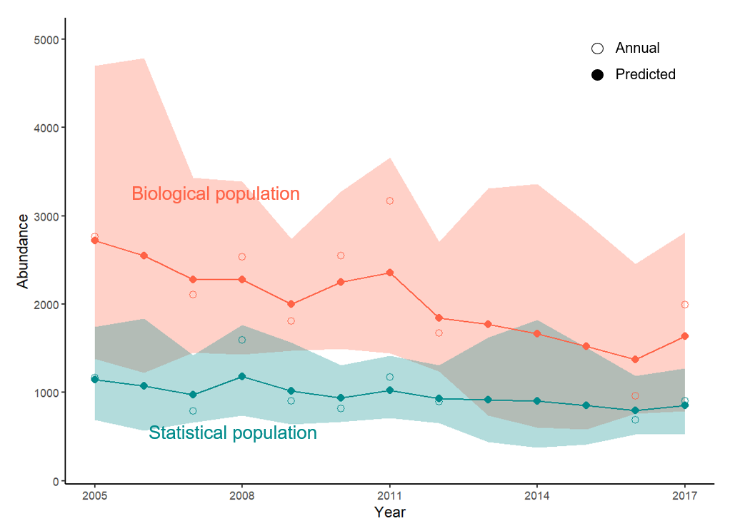
Figure 9 - Annual and predicted abundance estimates of the statistical population (without probability of presence, pp) and biological population (with pp) of Kittlitz’s murrelets, Icy Bay, Alaska, 2005–2017. Annual estimates are denoted with open circles and predicted estimates from the state-space model are identified with closed circles; the shaded areas describe the 95% credible intervals of the modeled abundance. Pp is accounted for in the biological population estimates using telemetry data surrounding a 3-day window of a boat survey.
Discussion
We developed a contemporary modeling framework to account for a population misalignment and generate unbiased abundance estimates of a highly mobile, non-territorial species, the Kittlitz’s murrelet, in a dynamic marine environment. By decomposing detection probability, we were able to use multiple datasets of different data types that did not rely on replicate or repeat sampling, which was not feasible for our study species or area without an unrealistically large number of sampling occasions or sites (e.g., N-mixture models; Royle, 2004; Barker et al., 2018; Hostetter et al., 2019). Alternatively, we would have needed to devise a way to increase capture probabilities to utilize capture-recapture or resight models effectively (Burnham et al., 1987). Moreover, the hierarchical structure of our model allowed us to work within a single analytical framework and appropriately account for multiple sources of uncertainty.
We are not aware of another abundance model that accounts for all components of detection probability, especially the probability of presence (pp), without using replicate or repeat sampling methods. Fischbach et al. (2022) developed a similar ratio estimator to account for haulout probability, which is analogous to pp, for estimating abundance of Pacific walrus, a species like Brachyramphus murrelets for which population monitoring is notoriously difficult. Their model combined count data from unoccupied aircraft systems and telemetry data, and therefore, while conceptually similar to our approach, it is not applicable to our situation because of differences in data types and habitat dynamics, nor does it account for the other components of detection probability. In these ways, our model builds on that of Fischbach et al. (2022) and adds to the toolbox of demographic models that account for spatial temporary emigration. While our modeling framework could be used for any species and in any system, it is most useful when repeat or replicate sampling is not practical, such as for species with low recapture and resight rates (e.g., nomadic raptors), species sampled during non-territorial portions of their annual cycle (e.g., wintering concentrations of ungulates), and species that occupy dynamic habitats (e.g., coral reef fishes).
By accounting for pp in our model, which aligned the statistical and biological populations, we improved the precision of annual abundance estimates for Kittlitz’s murrelets by 13–35% when we followed our standard protocol of conducting two boat surveys. However, results from 2009, when only one boat survey was conducted, clearly indicated that pp and survey effort were conflated, as the CV for the abundance estimate increased about tenfold. This outcome emphasizes the importance of a second boat survey annually if pp varies; otherwise, the abundance estimate from a single survey can have misleadingly high precision. We suspect this implication would be true for other highly mobile species and dynamic systems as well. Nonetheless, our ability to notably improve CVs for abundance estimates is a major achievement for a species often plagued with imprecise estimates (USFWS, 2013; Hoekman, 2019).
Although we increased the precision of annual abundance estimates by aligning the statistical and biological populations, we did not see the same improvement in the estimate of mean r, or temporal trend. Thus, while we explained and reduced variation in abundance within a year, we failed to account for a source(s) of variation across years. We may have gained some precision in the trend estimate by running a dynamic (multi-year) model instead of a static (single-year) model, though we suspect it would have been minimal. We think most of the variation in trend relates to the propensity for Kittlitz’s murrelets to skip breeding in some years and resultant variable return rates to Icy Bay. In fact, our recent integrated population model for this species, which accounted for non-breeding behavior, reduced uncertainty of the temporal trend estimate by 85% (Kissling et al., In revision). It is worth noting that while we did not increase precision of the trend estimate with our model described here, we also did not reduce it even though we added a parameter to the estimation process, suggesting some information about pp was useful.
Though a population misalignment existed, we found that abundance estimates for the statistical population of Kittlitz’s murrelets in Icy Bay generally were proportional to those of the biological population. We were somewhat surprised by this finding because, based on a survival analysis with the same telemetry dataset, radio-tagged murrelets moved frequently among spatial states with daily transition probabilities ranging from 0.135 to 0.279 (Kissling et al., 2015b). Yet, despite these moderate movement rates, pp varied little within a year (Figure 5). Further, pp was correlated with abundance of the statistical population across years (Figure 7), which suggests that murrelets in our study area were operating as a single biological population, otherwise we would have expected discordance. Importantly, we did not detect a temporal trend in pp, the link between the two types of populations, meaning that pp in the statistical population was random with respect to the biological population and inference could be extended without bias.
As with all models, our model has assumptions beyond those associated with specific methods like radio telemetry (White & Garrott, 1990) and distance sampling (Buckland et al., 2001). Inherent to boat and telemetry surveys, we assumed that the statistical population was closed with respect to pp for survey duration and within the 3-day window used to estimate biological population abundance. While we developed our model in part to avoid assumptions of closure, it is not entirely possible with the survey methods used in our study; essentially, our model relaxed the assumption considerably, though did not eliminate it. Even so, given that estimates of pp did not vary much within a year, we feel confident that we sufficiently met the closure assumption for the purpose of estimating abundance. For trend estimation, we also assumed that mean pp was an adequate estimate of pp in the three years with boat survey data but without telemetry data. Given that pp varied considerably across years, this assumption likely was violated, but in the absence of annual telemetry data, we think that the mean and its associated variance are adequate because the variance was correctly incorporated into the trend variance by the Bayesian model. Also, when estimating pk, we assumed that both murrelet species were equally likely to be classed as unidentified. We think this assumption was met reasonably well in our dataset even though Kittlitz’s murrelets far outnumber marbled murrelets in our study area. Further, using field trials, we found misidentification rates of Brachyramphus murrelets to be low (Schaefer et al., 2015).
Our final assumption was that the tagged murrelets were representative of the biological population, as we defined it. Although our boat surveys were conducted in early July, we tagged murrelets in May because our capture technique requires darkness, which is not sufficiently available in our study area for about 6–8 weeks surrounding summer solstice (21 June). Therefore, we inevitably tagged a few birds that were transiting through Icy Bay, which we only located once or twice, or never again. These birds were not included in our estimation of pp because they were not located during our boat surveys, so they are not relevant here. Additionally, because we only conducted telemetry flights in the Icy Bay study area, it is possible that some tagged birds could have temporarily emigrated beyond our search area, which would have biased our estimation of pp. However, we do not believe it was the case, largely because it was rare for a tagged bird to leave our study area and then return, especially as late in the breeding season as July. In fact, we removed eight locations (<2%) from our analysis because they were not within any of the five spatial states; none of those birds were located again, suggesting they permanently emigrated, or possibly the tag stopped reporting for whatever reason. Therefore, we feel confident this assumption was met as best we could with VHF transmitters.
Despite our poor ability to predict pp from environmental covariates, we gained new insights into the ecology of Kittlitz’s murrelets. First, in previous studies of this species, we posited that, if murrelets temporarily emigrated during boat surveys, they were moving into dense icefloes near the tidewater glaciers (i.e., Upper Bay), presumably to search for food or avoid predation (Kissling et al., 2007; Day et al., 2020). Here, we confirmed that when the proportion of ice in the Icy Bay state increased, pp decreased, but we found that instead of moving into pack ice closer to the glacier(s), murrelets moved into shallow or rough waters away from the glaciers (i.e., East Bay and Ocean, respectively). While this finding should be viewed cautiously until confirmed at other times and locations, it appears that murrelets are less associated with ice when at sea at fine spatial scales than we previously thought, at least in the Icy Bay system.
Second, although pp varied little within a year, it varied considerably across years, revealing a spatiotemporal pattern that implied an ecological driver(s) was at play but was not captured by the available environmental covariates. For example, pp was comparatively low across the 15-day period in 2007 and 2010, yet in 2007, murrelets outside of the sampled area were mostly in the Ocean state and in 2010, they were mostly in the East Bay state (Appendix 2). From this result, we assume that variation in prey availability led murrelets to select states outside of the Icy Bay state, with patterns that varied on an annual, rather than a within-year, basis. With additional data on murrelet movements from Icy Bay or elsewhere, this finding may eventually provide clues as to the ecological driver(s) of these patterns and improve our ability to predict pp.
Our modeling framework to align statistical and biological populations for abundance estimation is simple, flexible, and scalable and is suitable for a variety of species and habitats. It is a practical solution to resolving a population misalignment when repeat and replicate sampling is not feasible and increased precision of abundance and trend estimates is desired, as is the case with many species of conservation concern like the Kittlitz’s murrelet (USFWS, 2013). Although it requires telemetered animals, which can be costly compared to methods for unmarked animals, it was the only reasonable way to estimate pp for Kittlitz’s murrelets in Icy Bay and we suspect the same is true for other species and habitats that are difficult to sample (e.g., walrus; Fischbach et al., 2022). The use of satellite transmitters, which are not readily available yet for murrelets, would greatly facilitate and perhaps improve estimation of pp, especially if location data could be collected at a finer temporal scale. Moreover, satellite transmitters would relax the assumption related to representativeness of the tagged animals of the biological population and could improve precision of trend estimates if their retention and operation extended beyond a single year.
For any study reporting abundance, it is critical to clearly define the population to which abundance refers (Hammond et al., 2021), though delineating populations can be difficult and require substantial data (Rushing et al., 2016). Our goal here was not to provide a framework for how to delineate biological populations, but instead to develop an analytical approach to account for a population misalignment if one exists. However, we urge ecologists to think critically about the population in which they want to draw inference, especially as tracking technology improves and model complexity increases. If possible, the statistical population should be the same as the biological population, or at least representative of it in terms of population processes or ecological conditions, which fortunately happened in our case. Otherwise, if pp has temporal or geographic patterns, inference about abundance for the population of interest is confounded with its use of the sampled area and could be misleading. This messy situation with potentially misleading estimates can have conservation implications if threats or stressors vary. For example, threatened grizzly bears (Ursus arctos) can roam outside of national park boundaries, with bears outside the park being subject to differing mortality sources not captured by within-park monitoring (Schwartz et al., 2010). Further, if estimates of abundance are subsequently used in population models, it is imperative that they are from the same population used to estimate other demographic parameters (e.g., survival and productivity) to avoid misleading inference about population dynamics.
Acknowledgements
We are grateful for the field teams in Icy Bay, 2005–2017. In particular, we acknowledge Steve Lewis, Jonathan Felis, Nick Hatch, Sarah Schoen, Joe McClung, Leah Kenney, Nick Hajdukovich, Anne Schaefer, and Jon Barton. We thank Alsek Air and Icy Bay Lodge for logistical support and Tracy Gotthardt and Bill Hanson for administrative support. Many thanks to Josh Schmidt, Jim Nichols, and Rebecca Taylor for helpful conversations during analysis. Scott Mills, Rob Suryan, Sarah Sells, and Josh Millspaugh provided comments on earlier drafts of this manuscript, for which we are eternally grateful. We graciously acknowledge and respect that Icy Bay and the lands that surround it are within the traditional territories of the Yakutat Tlingit Tribe. Preprint version 3 of this article has been peer-reviewed and recommended by Peer Community In Ecology (https://doi.org/10.24072/pci.ecology.100640; Souchay, 2024).
Funding
We conducted this study with primary assistance from the U.S. Fish and Wildlife Service, National Park Service (Wrangell-St. Elias National Park), Alaska Department of Fish and Game (ADFG), and University of Montana. ADFG provided funding for data analysis and publication.
Conflict of interest disclosure
The authors declare no conflict of interest.
Data, scripts, code, and supplementary information availability
All data collected between 2005 and 2012 that were used in this manuscript, appendices, and annotated code used for analysis are publicly available (https://doi.org/10.5061/dryad.0cfxpnw8m; Kissling et al., 2024a). However, boat survey data from 2016 and 2017 were collected by the Alaska Department of Fish and Game, who considers these data to be sensitive and has withheld them in accordance with Alaska State Statute 16.05.815(d). Request of these data can be made to: Wildlife Science Director, Alaska Department of Fish and Game, Division of Wildlife Conservation, 1255 West 8th St., Juneau, Alaska, 99802 or to dfg.dwc.director@alaska.gov.