

 CC-BY 4.0
Introduction
The understory, comprising all woody and non-woody vascular plants under the tree canopy that rarely exceed two meters in height (Balandier et al., 2022a), is often overlooked despite its ecological importance to forest dynamics, carbon and nutrient stocks, and ecosystem functioning (Gonzalez et al., 2013; Haritika & Negi, 2025). The contribution of understory biomass to total forest biomass varies greatly among climatic regions and forest types (Jin et al., 2022), and is mainly influenced by the availability of resources and surrounding environmental conditions. Though the understory biomass generally accounts for less than 6% of the total biomass in temperate forests and for 3% in tropical forests (Battles, 2021; Brown, 1997; Jin et al., 2022), understory leaf biomass can be equivalent to overstory leaf biomass (Landuyt et al., 2020b). Understory plants also contribute significantly to ecosystem energy, water and nutrient fluxes (Balandier et al., 2022b), affect forest regeneration dynamics (Balandier et al., 2006), constitute habitats, food and shelter for other organisms (Landuyt et al., 2019) and are an important reservoir of forest biodiversity (Gilliam, 2007). A recent review also underlines that overstory-understory interactions are not unidirectional but act in both ways with complex pathways through the facilitation and competition for light, water, and nutrients (Balandier et al., 2022b) and interact with large-scale disturbances such as fire and large herbivores (Lecomte et al., 2024) to govern species coexistence and ecosystem dynamics.
Thanks to its multiple ecological functions, the understory is a key stratum in shaping the structure and functioning of forest ecosystems. Consequently, accurately quantifying understory attributes is essential in order to understand forest dynamics and ecological processes. Community diversity describes the understory composition, while biomass serves as a proxy for ecosystem functioning and resource availability. Thus, in studies of forest regeneration, the understory biomass has been used to quantify the vegetation that facilitates or compromises the establishment of seedlings (De Lombaerde et al., 2021). It also makes it possible to assess the quantity of fine fuels in fire risks (Lecomte et al., 2024). Moreover, in studies of biogeochemical cycles, quantifying aboveground biomass made it possible to estimate the input and stock of organic matter and nutrients (Landuyt et al., 2020a). While in some studies, the vegetation cover by species or group of species is sufficient (Thomas et al., 1999; Didham et al., 2005; Maillard et al., 2021), other studies relied on understory biomass values (Bolte, 2006). Several methods are used to estimate biomass, which differ in cost, field effort, data analysis, accuracy, species, and components of biomass required. These methods were reviewed by Catchpole & Wheeler (1992), who grouped them into direct sampling methods, calibrated visual estimation methods, and double sampling methods, as developed in the following paragraphs.
Destructive sampling is a direct sampling method that involves harvesting all vegetation to measure biomass. The advantage of this method is its accuracy, as it is a direct measure of biomass at a particular sampling point. However, the sampling must be representative of the study area. This method is time-consuming and destructive, disturbing ecological processes and influencing future outcomes, especially in time-series studies. It is generally used as a reference and a calibration standard for other types of methods.
Non-destructive methods, whose main advantage is the avoidance of degrading the studied areas, are traditionally based on calibrated visual estimations (Catchpole & Wheeler, 1992). This method consists of visually estimating biomass directly in situ. The method requires calibration by the observer based on several quadrat samples. Qualified observers can estimate vegetation mass with an accuracy of about 90%, but efficiency and bias depend on the observer and the spatial variability of the vegetation (Catchpole & Wheeler, 1992). Another non-destructive method for estimating biomass that is less susceptible to observer effects is the point-intercept method (Jonasson, 1988), which involves recording plant contacts along vertical lines at regular intervals along a transect or within a quadrat.
The double sampling method requires only a few field samples and measurements to build allometric equations that accurately estimate biomass with minimal destruction and relatively rapid results. Allometric equations make it possible to calculate biomass from simple and reproducible measurements. The approach is flexible and can be adapted to a wide range of ecological objectives and plant species from herbaceous species (Tackenberg, 2007; Pottier & Jabot, 2017) to trees (Bréda, 2003; Hays et al., 2020). For instance, it was used by Bréda (2003) to estimate leaf area index (LAI) in dominant trees. Several studies have developed allometric biomass models based on photographs of vegetation taken in the field followed by pixel-based image analysis (Paruelo et al., 2000; Tackenberg, 2007; Hays et al., 2020). For very large areas, biomass can be estimated from airborne LIDAR (Light Detection and Ranging) images (Estornell et al., 2011; Roth & Streit, 2018). This has the advantage of not being subject to observer effects, and allowing large areas to be covered in a short time. With a few height measurements in the field, the understory layer can be separated from the other forest strata (Ducey & Astrup, 2018). However, the calculated biomass represents the total biomass of the stratum without distinguishing among the species present, although this is a promising development direction. This method also has the disadvantage of requiring expensive equipment, and tedious and complex data processing. Field-measurements combined with allometric equations is still the most used and cheapest method, and transferable between contrasted environments (Pottier & Jabot, 2017).
In this study, allometric equations are used to calculate biomass from cover and height, or from phytovolume, combining both of these measurements (Porté et al., 2009; Pottier & Jabot, 2017). The double-sampling method can be applied to groups of understory plants (Bolte, 2006) as well as to species (Bolte, 1999; Gonzalez et al., 2013). The models for aboveground biomass estimation found in the literature were created at the local (Gonzalez et al., 2013) or regional level on different soils and types of temperate forest (Bolte, 1999, 2006).
To our knowledge, no previous studies have compared different plant cover estimation methods (i.e., two visual estimations and one systematic measurement) for biomass modelling, yet developing models for multiple cover estimation methods might add to the accuracy of the models and be useful for grouping protocols that do not use the same methods.
Besides total biomass, leaf and stem biomass and the allocation partitioning are often of interest. Separating leaf and stem biomass is essential especially for researchers attempting to model carbon and nutrient allocation (Litton et al., 2007), to study input of organic matter and nutrients to soil through litter fall (Landuyt et al., 2020a), to study the response of vegetation to biotic (herbivory) (Fan et al., 2019) or abiotic (drought, light) factors (Poorter et al., 2012), or to quantify the availability of food resources for animals (Borkowska & Konopko, 1994). Biomass allocation can be derived from the allometric partitioning theory, which is based on the metabolic scaling theory of (West et al., 1999), following the equation:
-
\(M_{y} = \ \alpha \bullet {M_{x}}^{\beta}\)
where Mx and My are the biomass of different organs, α is a species-specific normalization constant and β is the allometric scaling exponent (West et al., 1997; Enquist & Niklas, 2002). The vast majority of organisms (animals, plants, microbes) exhibit a scaling exponent very close to 0.75 according to the metabolic scaling theory. For plants, the theory was first developed and tested for tree species, confirming the theoretical scaling exponent. Then, later work showed that the exponent was equal to or very close to 1 for small or non-woody plants (Niklas, 2006). The scarcity of data on understory species is an important knowledge gap because allometric partitioning theory considers that plant size is the primary driver of biomass allocation patterns (Enquist & Niklas, 2002).
In this study, based on the double sampling method, we aim to develop models to estimate aboveground biomass (total, leaf, and stem) and provide allometric partitioning equations for leaf and stem biomass of widely represented understory plants in French and European temperate forests, with varying ecologies, botanical families and morphologies. Six species were thus sampled: wood anemone (Anemone nemorosa L.), common heather (Calluna vulgaris (L.) Hull), common honeysuckle (Lonicera periclymenum L.), purple moor-grass (Molinia caerulea (L.) Moench), common bracken (Pteridium aquilinum (L.) Kuhn) and brambles (Rubus fruticosus agg. L.).
The objectives of the study were to:
-
Create straightforward and reproducible allometric biomass models based on parameters that are easily measured in situ, including cover and height.
-
Determine the best allometric equation for each species.
-
Determine the most accurate of the three different plant cover estimation methods.
-
-
Determine the constant α and the allometric scaling exponent β in the allometric partitioning equations and assess the leaf-to-stem ratio.
Materials and methods
Study sites
The 21 study sites were located in both lowland (14 sites) and mountainous (7 sites) areas in France, with altitudes ranging from 55 m to 300 m for the lowland sites and from 700 m to 1300 m for the mountain sites. The forest stands were dominated by sessile oak (Quercus petraea (Matt.) Liebl.) in the lowlands and silver fir (Abies alba Mill.) in the mountains (Table 1 and Figure 1). Oak stands were 121 ± 26 years old, and silver fir stands were 117 ± 21 years old. Most of the forest stands were managed as even-aged high forests, while some were managed as coppice with standards or uneven-aged forests. Stand basal area was calculated from tree inventory data using diameter at breast height measurements. Stand age was estimated by dendrochronological analysis (tree core sampling) from a subsample of overstory trees within each stand (see footnotes in Table 1). The study sites were located on various soil types, from extremely to slightly acidic soils, classified according to the World Reference Base soil classification system (IUSS Working Group WRB, 2015) (Table 1). Soil pH was measured in systematic and representative soil samples in the first 10 cm of the mineral soil. All the sites were located in the temperate climate zone: in the mountain sites, the mean annual temperature ranged between 6.3 and 9.8°C and the annual precipitation between 1108 and 1723 mm, while in the lowland the annual mean temperature ranged between 10.2 and 12.0°C and the annual precipitation between 707 and 1032 mm (Table 1).
Sampling of studied understory species
We studied six understory species that are common and widespread in European temperate forests, representing different morphological, biological and ecological characteristics (Table 2): Anemone nemorosa L. (wood anemone), Calluna vulgaris (L.) Hull (common heather), Lonicera periclymenum L. (common honeysuckle), Molinia caerulea (L.) Moench (purple moor-grass), Pteridium aquilinum (L.) Kuhn (common bracken) and Rubus fruticosus agg. L. (brambles). These six species are widespread, occupying over more than 50% of the European territory (Grime et al., 2007): 74% for A. nemorosa, 77% for C. vulgaris and M. caerulea, 49% for L. periclymenum, 92% for P. aquilinum and 87% for R. fruticosus agg.
For R. fruticosus agg. and the climbing species L. periclymenum, tall shrubs and trees were avoided and only creeping plants or those climbing on other low-growing understory plant species.
Following a visual pre-assessment of plant cover at study sites, quadrats were strategically placed to capture the full range of cover gradients present at each site. At each site, quadrats were spaced at least five meters apart to reduce spatial autocorrelation. In this way, we ensured a complete coverage of plant cover (from 1% to almost 100%) and heights across study sites and forest types. At sites 9, 13 and 19, we measured and took ten samples of C. vulgaris, M. caerulea, and P. aquilinum, and 30 samples of A. nemorosa, L. periclymenum, and R. fruticosus agg. For logistical reasons, we were unable to conduct the same sampling effort at the other sites, and reduced to four samples of each species when present and sometimes less when small and scattered presence. In total, we obtained 42 samples of A. nemorosa, 16 of C. vulgaris, 75 of L. periclymenum, 27 of M. caerulea, 45 of P. aquilinum, and 103 of R. fruticosus agg. (Figure 1 and Table 3).

Figure 1 - Sampling design of the study. The sites (numbered from 1 to 21, Table 1) are located with symbols showing where the different understory species (Anemone nemorosa, Calluna vulgaris, Lonicera periclymenum, Molinia caerulea, Pteridium aquilinum, Rubus fruticosus agg.) were sampled. Symbol colour shows the associated type of forest: stands dominated by silver fir, Abies alba or sessile oak, Quercus petraea. Symbol size represents the number of samples per study site.
Biometrical measurements and biomass sampling of understory species
We sampled understory plants beneath forest canopies and harvested them during the peak of plant development in July and August 2023 and 2024 for C. vulgaris, L. periclymenum, M. caerulea, P. aquilinum, and R. fruticosus agg. (Gimingham, 1960; During et al., 1994; Taylor et al., 2001; Marrs & Watt, 2006; Taylor, 2005), and in April 2024 for A. nemorosa (Mårell et al., 2009). We estimated the plant cover, measured the height, and collected the living vegetative aboveground parts of the sampled plants (stems and leaves) in 0.5 m2 quadrats (71 × 71 cm). For all measurements and sampling, only stems and leaves were taken into account and we discarded inflorescences, fruits, seeds, and dead parts.
Table 1 - Study site stand and pedo-climatic characteristics: main tree species, soil type, pH, annual mean temperature (°C), annual cumulative precipitation (mm) for the 1991-2020 period, altitude (m), forest management type, tree age (year), stand basal area (m2 ha-1) and other main tree species (in descending order of dominance and > 10% of the total basal area). NA stands for ‘not available’
|
Forest type |
Main tree species |
Forest id |
Soil type |
pH water |
Temp. (°C) |
Precip. (mm) |
Altitude (m) |
Forest management type |
Tree age (yr) |
Basal area (m2 ha-1) |
Other main tree species |
|---|---|---|---|---|---|---|---|---|---|---|---|
|
Mountain forest |
Abies alba |
1 |
Cambisol |
4.5 |
7.4 |
1558 |
1100 |
Even-aged |
123 a |
35 a |
- |
|
2 |
4.5 |
8.9 |
1263 |
400 |
Even-aged |
83 a |
38 a |
Picea abies |
|||
|
3 |
4.9 |
7.3 |
1611 |
680 |
Even-aged |
133 a |
49 a |
- |
|||
|
4 |
Cambisol and leptosol |
5.7 |
6.3 |
1723 |
1000 |
Uneven-aged |
110 a |
50 a |
Picea abies |
||
|
5 |
5.4 |
8.0 |
1371 |
1150 |
Uneven-aged |
149 a |
30 a |
Fagus sylvatica |
|||
|
6 |
Luvisol |
6.2 |
9.8 |
1108 |
950 |
Even-aged |
109 a |
46 a |
- |
||
|
7 |
Podzosol |
4.3 |
6.3 |
1444 |
1300 |
Even-aged |
109 a |
51 a |
- |
||
|
Lowland forest |
Quercus petraea |
8 |
Cambisol |
4.7 |
11.3 |
1032 |
260 |
Even-aged |
117 a |
31 a |
Carpinus betulus |
|
9 |
5.3 |
11.0 |
707 |
120 |
Coppice with standards |
105 b |
NA |
Carpinus betulus |
|||
|
10 |
Cambisol and planosol |
4.5 |
11.2 |
820 |
260 |
Even-aged |
144 a |
32 a |
- |
||
|
11 |
Planosol |
4.6 |
10.1 |
905 |
315 |
Even-aged |
114 a |
32 a |
Carpinus betulus |
||
|
12 |
4.6 |
10.5 |
713 |
55 |
Even-aged |
89 a |
27 a |
Carpinus betulus |
|||
|
13 |
4.5 |
10.9 |
749 |
150 |
Even-aged |
83 c |
20 c |
Pinus sylvestris |
|||
|
14 |
Planosol and luvisol |
4.5 |
11.2 |
834 |
180 |
Even-aged |
107 a |
30 a |
- |
||
|
15 |
Luvisol |
4.9 |
10.9 |
839 |
220 |
Even-aged |
116 a |
31 a |
- |
||
|
16 |
4.4 |
11.3 |
669 |
130 |
Even-aged |
121 a |
34 a |
Fagus sylvatica |
|||
|
17 |
4.7 |
12.0 |
925 |
300 |
Even-aged |
127 a |
29 a |
- |
|||
|
18 |
4.5 |
10.8 |
803 |
160 |
Even-aged |
112 a |
26 a |
- |
|||
|
19 |
5.1 |
10.9 |
713 |
150 |
Coppice with standards |
≈100 |
23 d |
Carpinus betulus |
|||
|
20 |
Podzol |
4.2 |
10.2 |
892 |
180 |
Coppice with standards |
168 a |
30 a |
Fagus sylvatica Betula pendula |
||
|
21 |
Calcisol |
4.7 |
10.4 |
851 |
260 |
Coppice with standards |
166 a |
16 a |
Carpinus betulus Tilia cordata |
a Stand basal area was calculated from eight 500 m2 subplots tree inventory data using diameter at breast height measurements. Stand age was estimated by dendrochronological analysis from a subsample of 30 overstory trees. b Stand age corresponded to the mean age of the sampled plots, obtained from the forest management plan. c Stand basal area was calculated from full tree inventory data using diameter at breast height measurements. Stand age was estimated by dendrochronological analysis from a subsample of 18 overstory trees. d Stand basal area was calculated from full tree inventory data using diameter at breast height measurements and including only the stems of the dominant tree species (Quercus petraea) with a diameter above 17.5 cm, excluding Carpinus betulus coppice stems.
Table 2 - Morphological characteristics, life form, life cycle and autecology of the six studied understory species
|
Species |
Life form (Raunkiær system) |
Morphology |
Life cycle |
Autecology |
|---|---|---|---|---|
|
Anemone nemorosa |
Geophyte |
Forb. Acaulescent plant. Branched rhizome. Erect stem. Palmately lobed leaves and bracts. |
Perennial. Early life cycle. Deciduous leaves. |
Shade tolerance. Acidophilous to calcicolous. Mesic. |
|
Calluna vulgaris |
Chamaephyte |
Dwarf shrub. Caulescent plant. Woody branched stems. Small xeromorphic leaves. |
Perennial. Evergreen. |
Heliophilous or partial shade. Broadly acidophilous. Xeric to hygrophilous. |
|
Lonicera periclymenum |
Chamaephyte |
Shrub. Caulescent plant. Woody branched stems. Climbing or creeping twining plant. Oval hairy leaves. |
Perennial. Layering. Deciduous or semi-deciduous. |
Heliophilous or partial shade. Broadly acidophilous. Mesic to hygrophilous. |
|
Molinia caerulea |
Hemicryptophyte |
Graminoid. Acaulescent plant. Semi-rosette tussock. Linear leaves. |
Perennial. Deciduous leaves. |
Heliophilous or partial shade. Acidophilous. Mesic to hygrophilous. |
|
Pteridium aquilinum |
Geophyte |
Fern. Acaulescent plant. Frond arising from rhizome. |
Perennial. Deciduous leaves and stem. |
Heliophilous or partial shade. Broadly acidophilous. Xeric to hygrophilous. |
|
Rubus fruticosus agg. |
Phanerophytes |
Shrub. Caulescent plant. Arching or erect spiny semi-woody stems. Ternate or palmate leaves. |
Perennial. Layering. Biennial to perennial stems. Long-lived or persistent leaves through the winter in some taxa. |
Heliophilous. Moderately acidophilous. Mesic. |
Table 3 - Number of observations and descriptive statistics of projection cover (%) for each species according to forest type
|
Species |
Forest type |
Number |
Min |
Max |
Mean |
Standard deviation |
Coefficient of variation |
|---|---|---|---|---|---|---|---|
|
Anemone nemorosa |
Lowland |
39 |
1 |
98 |
31.6 |
27.8 |
88.0 |
|
Mountain |
3 |
1 |
8 |
3.7 |
3.8 |
102.7 |
|
|
Calluna vulgaris |
Lowland |
14 |
3 |
70 |
31.9 |
19.1 |
59.9 |
|
Mountain |
2 |
10 |
80 |
45.0 |
49.5 |
110.0 |
|
|
Lonicera periclymenum |
Lowland |
72 |
1 |
80 |
27.4 |
19.6 |
71.5 |
|
Mountain |
3 |
8 |
45 |
27.7 |
18.6 |
67.1 |
|
|
Molinia caerulea |
Lowland |
25 |
1 |
95 |
34.3 |
27.8 |
81.0 |
|
Mountain |
2 |
5 |
30 |
17.5 |
17.7 |
101.1 |
|
|
Pteridium aquilinum |
Lowland |
34 |
2 |
100 |
46.4 |
29.8 |
64.2 |
|
Mountain |
11 |
25 |
100 |
61.6 |
29.3 |
47.6 |
|
|
Rubus fruticosus agg. |
Lowland |
75 |
2 |
95 |
33.7 |
25.5 |
75.7 |
|
Mountain |
28 |
9 |
100 |
55.9 |
30.2 |
54.0 |
Plant cover
On field, we estimated three type of plant cover by (a) visual estimations of the plant cover envelope (coarse outline of the plant), (b) visual estimations of the projected plant cover (exact outline of the plant), and (c) systematic measurements following the point-intercept method using a metal rod of 4 mm in diameter and 36 points (Goodall, 1952) (Figure 2). For the point-intercept method, when the rod touched either the stem or a leaf, the species was noted present, whatever the number of contacts at the same point. The same observer carried out the visual estimates for all species and study sites to the nearest 5% to minimize any observer effect. The observer was trained on examples of known plant cover thanks to COVERater (Cruickshank et al., 2024).

Figure 2 - Schematic representation of the three plant cover estimation methods using a triangular frond of Pteridium aquilinum as an example: (a) envelope, (b) projection, and (c) point-intercept method. Green areas indicate the visually estimated cover for methods (a) and (b), while the green dots in (c) represent the points in contact with the plant. For the point-intercept method, the number of contacts was converted into percentage cover using a simple proportion (e.g., 12 contacts out of 36 points correspond to a cover of 33%).
Height
For each quadrat and species, the quadrat was divided into four quarters in which we measured the height of the tallest part of the studied plant species, whether it was a stem or a leaf, using a folding ruler with centimeter precision. The maximum height was measured without straightening the plant and even if the measurements came from different parts of the same individual. We then calculated the mean among the four maximum heights per quadrat to smooth out extreme height values.
Aboveground biomass
For woody and semi-woody plants (Table 2), we sampled all living leaves and stems from inside the quadrat. We cut the aerial parts at ground level and along the vertical edges of the quadrat when plant parts extended beyond the quadrat’s limits. Plant parts inside the quadrat were collected even if the plant was rooted outside. This approach was used because these species often exhibit extensive lateral branching and intertwined, layered shoots, which makes it difficult to identify the exact rooting position. Regarding herbaceous plants and ferns, we collected only those rooted within the quadrat. Thus, we collected plant parts outside the quadrat when the plant was rooted within it, and we did not collect plant parts inside the quadrat when the plant was rooted outside it. This method was preferred for herbaceous species because individual rooting points could be identified more reliably.
In the laboratory, the samples were oven-dried for 48 hours at 65°C and then weighed directly to an accuracy of 0.02 g. For the woody and semi-woody plants (C. vulgaris, L. periclymenum, R. fruticosus agg.), we separated the leaves (petiole included) and stems prior to oven drying. For C. vulgaris, as separating leaves and stems was a time-consuming task, we separated organs for only a part of each sample. To address the architectural variability observed among sites and individuals (e.g., proportion of stem and leafless parts due to age), we first separated the leafless stem sections from those with leaves. From the latter, we then defoliated 20% of the stems. This approach ensured that variability linked to architecture did not affect the subsample. Then, the leaf-to-stem mass ratio was applied to the rest of the subsample. Therefore, the leaf mass and the stem mass (sum of leafless stem and those with leaves) were obtained. For P. aquilinum, we separated the leaflet from the rachis of the frond, which was considered here as a stem. The total aboveground biomass was obtained by summing the dry weight of leaves and stems.
Data analysis and allometric models
Our objective was to determine the best models to estimate total (MT), leaf (ML), and stem (MS) aboveground biomass from simple field measurements of plant structure. The predictors tested included plant cover, plant height and phytovolume. Phytovolume (P, m3 ha-1), is a proxy of the three-dimensional space occupied by vegetation. It was calculated following Porté et al. (2009):
-
\(P = C \bullet H\)
where C is the plant cover (%) and H is the average maximum height of the plant (cm). Models were tested separately for each species. We tested linear (Eqn. 3), second-degree polynomial (Eqn. 4), and power (Eqn. 5 and 6 used by Gonzalez et al. (2013) and Bolte (2006), respectively) scaling relationships with plant cover, average maximum height of plant or phytovolume:
-
\(M = a \bullet \ v\)
-
\(M = a \bullet {v\ }^{2} + \ b\ \bullet v\)
-
\(M = a \bullet {v\ }^{b}\)
-
\(M = a \bullet C^{b} \bullet {H\ }^{c}\)
where M is biomass in g m-2, \(v\) is any plant cover (C) in % or phytovolume (P) in m3 ha-1, H is the average maximum height of plant in centimeters, and a, b, and c are coefficients. The models were fit using the R Statistical Software (version 4.4.2).
We used weighted nonlinear least squares to fit scaling relationships between biomass and the allometric metrics (plant cover, height, and phytovolume) in order to adjust for the unbalanced sampling design (weighted proportionally to the number of quadrats per species and per study site) and to correct for heteroscedasticity, this means reducing the disproportionate influence of the most variable observations (weights argument in nlsLM function, minpack.lm R package, Elzhov et al., 2023). We ran five types of weights for each model: (i) the weight for sampling design alone, (ii) the weight for sampling design and the inverse response (a higher biomass results in a lower weight), (iii) the inverse fitted (less impacted by outliers and a higher biomass results in a lower weight), (iv) the inverse squared fitted (less impacted by outliers and a higher biomass results in a much lower weight), or (v) the inverse squared residuals (a variable biomass results in lower weight). We therefore tested and compared 21 models per species (7 scaling relationships × 3 cover methods) across the five types of weights, resulting in a total of 105 models per species and compartment (total aboveground, leaf, stem). To assess the best model and best cover methods for each species, we used three sequential criteria. (1) First, we retained the models that obeyed the hypotheses of normality of residuals and homoscedasticity using the Shapiro and the Breusch-Pagan tests at p-value 0.01 (lmtest R package, Hothorn et al., 1999), as this provides an objective and reproducible statistical evaluation compared with subjective visual inspection. (2) Then, we selected the best models based on the AICc (Akaike Information Criterion, corrected for small sample sizes). (3) Finally, when differences in AICc were lower than two, indicating models of similar explicative support, among the most parsimonious models, we chose the model with the lowest MSE (mean square error). AICc indicates the accuracy and simplicity of the model, while MSE evaluates its precision. We calculated the MAE (mean absolute error) and RMSE (root mean square error) to assess the models’ predictive ability. For the best model for each species, confidence intervals of the predictions were estimated using bootstrapping (n = 1000; modelr R package, Wickham, 2023).
As site and bioclimatic conditions varied greatly among the two forest types, we expected the latter to be a discriminating covariate. We therefore also tested the effect of forest type on a, b and c coefficients in the best aboveground biomass models retained for species with sufficient and balanced sample sizes in both forest types, specifically P. aquilinum and R. fruticosus agg. (Table 3). More specifically, forest type was introduced as an interaction term on each coefficient (a, b and c when applicable), allowing each coefficient to vary between mountain and lowland forests. To select the best model (with or without forest type) we used the same criteria as for selecting the best biomass models.
To compare prediction errors (RMSE) among the three cover methods, we retained all aboveground biomass models that showed satisfactory residual patterns as identified through graphical inspection, even when the Shapiro test indicated slight deviations from normality. Indeed, because this test is very restrictive and is sensitive to sample size, it may reject models with visually acceptable residuals distribution. Graphical inspection was therefore considered to evaluate the practical relevance of deviations from normality. Moreover, linear model coefficients and predictions are generally robust with moderate departures from normality, whereas statistical inference values such as p-values and confidence intervals are more strongly affected (Schmidt & Finan, 2018).
Here, we stipulated that the total aboveground biomass was the sum of leaf and stem biomass, \(M_{T} = \ M_{L} + M_{S}.\) Because it has been shown that biomass allocation patterns obey the allometric scaling law of the form \(M_{y} = \ \alpha \bullet {M_{x}}^{\beta}\), where Mx and My are biomass of different organs, α is a species-specific normalization constant, and β is the allometric scaling exponent (West et al., 1997; Enquist & Niklas, 2002), we estimated the scaling exponents between leaf (ML) and stem (MS) biomass for the different species as follows:
-
\(M_{Li} = \alpha_{i}{{\bullet M}_{Si}}^{\beta_{i}} \leftrightarrow \log_{10}M_{Li} = \log_{10}\alpha_{i} + \beta_{i}\ \bullet \log_{10}M_{Si}\ \)
and tested for differences in the scaling exponents among species, i, using log-log linear relationships (Eqn. 7) and standardized major axis (SMA) regression analysis (smatr R package, Warton et al., 2012). For species with a scaling exponent equal to one (β = 1, for spermatophytes without or with few secondary tissues (Niklas, 2006)), the leaf-to-stem ratio is equivalent to the constant α for each species. Since \(M_{T} = \ M_{L} + M_{S}\) and \(M_{L} = \ \alpha \bullet {M_{S}}^{\beta}\) when β = 1, simple algebraic rearrangements allow leaf and stem biomass to be estimated from the total aboveground biomass as follows:
-
\(M_{L} = \frac{\alpha}{1 + \alpha} \bullet M_{T}\)
-
\(M_{S} = \frac{1}{1 + \alpha} \bullet M_{T}\)
where α is the constant from Eqn. 7 and MT can be replaced by the fitted equations for the total aboveground biomass (Eqn. 3-6). Eqn. 8 and 9 were not directly used in the analyses, but for convenience we present them here as they allow leaf and stem biomass to be derived from total aboveground biomass (and conversely to reconstruct total biomass from its components) when β = 1.
Results
Allometric models for aboveground biomass
Biomass allometric relationships
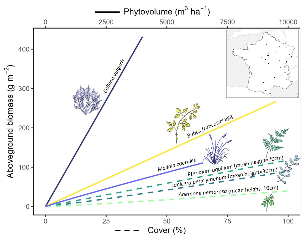
The plant cover gradient spanned the entire range of possible values, from 1% to almost 100%, for all six species. The total aboveground biomass ranged from 0.5 to 70 g m-2 for A. nemorosa, from 5 to 403 g m-2 for C. vulgaris, from 0.5 to 117 g m-2 for L. periclymenum, from 0.8 to 171 g m- 2 for M. caerulea, from 0.6 to 323 g m-2 for P. aquilinum and from 1 to 298 g m-2 for R. fruticosus agg.
The best models for total aboveground biomass were power functions of plant cover and height (Eqn. 6) for A. nemorosa, L. periclymenum, and P. aquilinum, power functions of phytovolume for M. caerulea, and a linear function (Eqn. 3) of phytovolume for C. vulgaris and R. fruticosus agg. (Figure 3 and Table 4). All of the best models included cover and height, which were either separate variables or included in the phytovolume. Including height in these models provided precision by up to 12% for P. aquilinum and R. fruticosus agg., and between 3 and 7% for A. nemorosa, C. vulgaris, and L. periclymenum, but did not improve precision for M. caerulea.
Forest type had no effect on the coefficients in the model for P. aquilinum, but had an effect in the model for R. fruticosus agg.: total aboveground biomass was 9% higher in the mountain and 5% lower in the lowland than biomass estimated with the model without forest type (Appendix S1). To compare consistent models across all species, we focused on models without forest type in subsequent analyses.

Figure 3 - Allometric relationships between total (MT) aboveground biomass (g m-2) and phytovolume (m3 ha-1) or cover (%) and height (cm) for (a) Anemone nemorosa (n = 42), (b) Calluna vulgaris (n = 16), (c) Lonicera periclymenum (n = 75), (d) Molinia caerulea (n = 27), (e) Pteridium aquilinum (n = 45) and (f) Rubus fruticosus agg. (n = 103). Points correspond to observed data, lines to model predictions, and the shaded areas to bootstrapped 95% confidence intervals. For C. vulgaris, the two models shown included all data (dashed gray line) or excluded (black line) an influential point (gray point). For models including height as explanatory variable, model predictions are shown for three quantiles of height (10%, 50% and 90%).
Table 4 - Best models for the allometric scaling relationship between total aboveground biomass (g m-2) for six species, as well as stem and leaf biomass for four species, and phytovolume (P in m3 ha-1) or cover (C in %) and height (H in cm). MT = total aboveground biomass, ML = leaf biomass, MS = stem biomass. Cover measure method, coefficients a, b, and c of the model, and p-value are given, as well as summary statistics
|
Formula |
Cover |
a |
b |
c |
p-value a |
p-value b |
p-value c |
Adjusted R2 |
MSE |
MAE |
RMSE |
|---|---|---|---|---|---|---|---|---|---|---|---|
|
Anemone nemorosa |
|||||||||||
|
MT = aCbHc |
Point-intercept |
0.0145 |
1.20 |
1.04 |
0.00049 |
<0.0001 |
<0.0001 |
0.88 |
25.80 |
3.68 |
5.08 |
|
Calluna vulgaris |
|||||||||||
|
MT = aP |
Projection |
0.108 |
- |
- |
<0.0001 |
- |
- |
0.79 |
3384 |
40.1 |
58.1 |
|
ML = aC + bC2 |
Projection |
2.48 |
-0.0131 |
- |
<0.0001 |
<0.0001 |
- |
0.36 |
498.1 |
17.8 |
22.3 |
|
MS = aP |
Envelope |
0.0514 |
- |
- |
<0.0001 |
- |
- |
0.79 |
1765 |
30.1 |
42.0 |
|
Lonicera periclymenum |
|||||||||||
|
MT = aCbHc |
Point-intercept |
0.247 |
1.10 |
0.244 |
0.0038 |
<0.0001 |
0.011 |
0.86 |
108.4 |
7.67 |
10.4 |
|
ML = aCbHc |
Point-intercept |
0.146 |
1.09 |
0.119 |
0.0053 |
<0.0001 |
0.24 |
0.83 |
17.25 |
3.03 |
4.15 |
|
MS = aCbHc |
Point-intercept |
0.112 |
1.13 |
0.305 |
0.012 |
<0.0001 |
0.0059 |
0.79 |
69.65 |
5.94 |
8.35 |
|
Molinia caerulea |
|||||||||||
|
MT = aPb |
Envelope |
0.027 |
0.948 |
- |
0.0079 |
<0.0001 |
- |
0.66 |
574.5 |
14.6 |
24.0 |
|
Pteridium aquilinum |
|||||||||||
|
MT = aCbHc |
Projection |
0.0211 |
1.00 |
0.932 |
0.19 |
<0.0001 |
0.0027 |
0.79 |
1330 |
21.9 |
36.5 |
|
ML = aCbHc |
Projection |
0.0159 |
1.47 |
0.473 |
<0.0001 |
<0.0001 |
<0.0001 |
0.74 |
721.3 |
15.8 |
26.9 |
|
MS = aPb |
Projection |
0.00302 |
1.04 |
- |
0.022 |
<0.0001 |
- |
0.79 |
155.3 |
6.94 |
12.5 |
|
Rubus fruticosus agg. |
|||||||||||
|
MT = aP |
Envelope |
0.0281 |
- |
- |
<0.0001 |
- |
- |
0.81 |
740.1 |
17.6 |
27.2 |
|
ML = aC + bC2 |
Point-intercept |
0.240 |
0.00641 |
- |
<0.0001 |
<0.0001 |
- |
0.85 |
124.7 |
7.81 |
11.2 |
|
MS = aCbHc |
Projection |
0.0132 |
0.836 |
1.22 |
0.0085 |
<0.0001 |
<0.0001 |
0.76 |
294.8 |
10.1 |
17.2 |
Cover estimation methods for biomass prediction
The best models included either point-intercept, projection, or envelope methods for estimating plant cover, depending on the species (Table 4). The best models for C. vulgaris and P. aquilinum were fitted using the projection cover, M. caerulea and R. fruticosus agg. using the envelope cover, and A. nemorosa and L. periclymenum using the point-intercept method. In this study, the three methods produced closely correlated cover estimates. The estimates of plant cover by envelope (Figure 2 (a)) and the point-intercept method (Figure 2 (c)) correlated with a unit-to-unit slope more closely (Pearson’s ρa,c = 0.95) than with projection (Figure 2 (b)) (ρa,b = 0.94 and ρc,b = 0.91, respectively) for which the slopes deviated from one.
Based on the best model for each species (Table 4), the other cover estimation methods are compared in Table 5 (for other total aboveground models, Appendix S2 and for leaf and stem models, Appendix S3). The differences in RMSE among cover methods were generally limited for R. fruticosus agg., L. periclymenum and P. aquilinum, with prediction errors differing by less than 10% between methods. In contrast, larger differences were observed for the other species, particularly for C. vulgaris and M. caerulea, for which the projection cover method produced lower RMSE values, with a reduction of up to 16% and 35%, respectively, compared with the envelope or point-intercept method. Considering all the models with visually satisfactory residual distributions, for each species and scaling relationship, comparisons among cover methods showed that 57% of models differed by less than 10% in prediction error, while 85% differed by less than 20% (Appendix S2).
The time to measure the visual envelope and projection cover was approximately one minute, while the time to measure the cover using the point-intercept method was around three to six minutes for the 36 points (depending on the cover, and included the phase of installing the point-quadrat).

Figure 4 - Allometric relationships between leaf, ML, and stem, MS, biomass (g m-2) for the following understory species: Calluna vulgaris (n = 16), Lonicera periclymenum (n = 75), Pteridium aquilinum (n = 45), and Rubus fruticosus agg. (n = 103). Reduced standardized major axis regression analysis of log10-transformed data (a) and back-transformed data (b). Points correspond to observed data, lines to model predictions, and the shaded areas to bootstrapped 95% confidence intervals.
Leaf-to-stem ratio
We investigated the leaf-to-stem ratio for C. vulgaris, L. periclymenum, R. fruticosus agg. and P. aquilinum. For P. aquilinum, the rachis was considered a stem, and the leaflets were considered leaves. The scaling exponents (β) for leaf (ML) against stem (MS) biomass were similar for C. vulgaris and L. periclymenum and did not differ from the expected isometric relationship (β = 1) (Figure 4 and Table 6). For these species, the coefficient α therefore represents the leaf-to-stem ratio, which remains constant regardless of the plant biomass. Contrarily, the scaling exponents for P. aquilinum and R. fruticosus agg., were below one and differed from the other species (Table 6). Consequently, the leaf-to-stem ratio was not constant and varied with plant biomass. For R. fruticosus agg. the scaling exponent was 0.8 which is close to the expected theoretical 0.75.
Similar patterns were observed between leaf and total aboveground biomass, and between stem and total aboveground biomass. Isometric relationships were found for most species, whereas R. fruticosus agg. showed a lower scaling exponent for leaf biomass and a higher scaling exponent for stem biomass with increasing total biomass. P. aquilinum also showed a slight increase in stem biomass allocation with increasing total biomass (Table 6).
In L. periclymenum and C. vulgaris, leaf biomass was lower than stem biomass (α < 1). Leaf biomass represented respectively 37% and 32% of the total aboveground biomass, corresponding to a constant leaf-to-stem ratio of 0.63 and 0.50, calculated directly from the measured biomass data ML and MS (equivalent to the constant α when β = 1, Table 6). For P. aquilinum, leaf biomass was greater than rachis biomass. It varied from 76% to 68% over the range of the sampled total aboveground biomass corresponding to a leaflet-to-rachis ratio varying from 2.1 to 3.2, also derived from observed biomass. For R. fruticosus agg., leaf biomass was greater than stem biomass at low values of total aboveground biomass (< 224 g m-2), while the inverse for higher values of total aboveground biomass (> 224 g m-2) (Figure 4). The leaf-to-stem ratio varied from 0.90 to 2.57 for R. fruticosus agg. over the range of the studied total aboveground biomass values.
Table 5 - Allometric scaling relationships for the six studied species between aboveground biomass (MT in g m-2) and cover (C in %), height (H in cm) or phytovolume (P in m3 ha-1) following normality of residuals and homoscedasticity (Shapiro test and Breusch-Pagan test p-values (in bold) or retained following visual inception of residual patterns). The cover measure method, coefficients a, b and c of the model and p-value are given, as well as R2, MSE, MAE, RMSE and AICc
|
Formula |
Cover |
a |
b |
c |
p-value a |
p-value b |
p-value c |
AICc |
Adjusted R2 |
MSE |
MAE |
RMSE |
p-value Shapiro test |
p-value Breusch-Pagan test |
|---|---|---|---|---|---|---|---|---|---|---|---|---|---|---|
|
Anemone nemorosa |
||||||||||||||
|
MT = aCbHc |
Point-intercept |
0.0145 |
1.20 |
1.04 |
0.00049 |
<0.0001 |
<0.0001 |
203.2 |
0.88 |
25.80 |
3.68 |
5.08 |
0.021 |
0.14 |
|
MT = aCbHc |
Projection |
0.115 |
0.938 |
0.729 |
0.065 |
<0.0001 |
0.00087 |
247.2 |
0.86 |
29.69 |
3.66 |
5.45 |
0.29 |
0.047 |
|
MT = aCbHc |
Envelope |
0.222 |
1.07 |
0.161 |
0.079 |
<0.0001 |
0.48 |
223.0 |
0.83 |
37.80 |
3.63 |
6.15 |
0.64 |
0.18 |
|
Calluna vulgaris |
||||||||||||||
|
MT = aP |
Projection |
0.108 |
- |
- |
<0.0001 |
- |
- |
147.0 |
0.79 |
3384 |
40.1 |
58.2 |
0.032 |
0.59 |
|
MT = aP |
Envelope |
0.072 |
- |
- |
<0.0001 |
- |
- |
177.3 |
0.73 |
4291 |
43.2 |
65.5 |
0.075 |
0.93 |
|
MT = aP |
Point-intercept |
0.0624 |
- |
- |
<0.0001 |
- |
- |
182.0 |
0.70 |
4694 |
49.1 |
68.5 |
0.0003 |
0.45 |
|
Lonicera periclymenum |
||||||||||||||
|
MT = aCbHc |
Point-intercept |
0.247 |
1.10 |
0.244 |
0.0038 |
<0.0001 |
0.011 |
566.2 |
0.86 |
108.4 |
7.67 |
10.4 |
0.094 |
0.025 |
|
MT = aCbHc |
Envelope |
0.231 |
0.888 |
0.479 |
<0.0001 |
<0.0001 |
<0.0001 |
582.6 |
0.82 |
136.4 |
8.54 |
11.7 |
0.091 |
0.55 |
|
MT = aCbHc |
Projection |
0.806 |
0.628 |
0.532 |
0.0055 |
<0.0001 |
<0.0001 |
601.7 |
0.83 |
126.1 |
8.34 |
11.2 |
<0.0001 |
0.33 |
|
Molinia caerulea |
||||||||||||||
|
MT = aPb |
Envelope |
0.027 |
0.948 |
- |
0.0079 |
<0.0001 |
- |
197.4 |
0.66 |
574.5 |
14.6 |
24.0 |
0.033 |
0.42 |
|
MT = aPb |
Projection |
0.0863 |
0.863 |
- |
0.28 |
<0.0001 |
- |
241.7 |
0.85 |
248.7 |
10.7 |
15.8 |
0.01 |
0.019 |
|
MT = aPb |
Point-intercept |
0.043 |
0.899 |
- |
0.37 |
<0.0001 |
- |
242.3 |
0.65 |
595.6 |
15.9 |
24.4 |
0.013 |
0.37 |
|
Pteridium aquilinum |
||||||||||||||
|
MT = aCbHc |
Projection |
0.0211 |
1.00 |
0.932 |
0.19 |
<0.0001 |
0.0027 |
406.7 |
0.79 |
1330 |
21.9 |
36.5 |
0.022 |
0.10 |
|
MT = aCbHc |
Point-intercept |
0.000484 |
1.97 |
0.789 |
0.57 |
0.0002 |
0.0017 |
448.9 |
0.79 |
1326 |
22.9 |
36.4 |
<0.0001 |
0.056 |
|
MT = aCbHc |
Envelope |
0.0003 |
1.55 |
1.26 |
0.45 |
0.0002 |
<0.0001 |
418.3 |
0.75 |
1529 |
23.3 |
39.1 |
0.0027 |
0.21 |
|
Rubus fruticosus agg. |
||||||||||||||
|
MT = aP |
Envelope |
0.0281 |
- |
- |
<0.0001 |
- |
- |
858.4 |
0.81 |
740.1 |
17.6 |
27.2 |
0.13 |
0.95 |
|
MT = aP |
Point-intercept |
0.0296 |
- |
- |
<0.0001 |
- |
- |
875.5 |
0.79 |
799.1 |
18.0 |
28.3 |
0.033 |
0.21 |
|
MT = aP |
Projection |
0.0331 |
- |
- |
<0.0001 |
- |
- |
769.7 |
0.82 |
681.3 |
17.6 |
26.1 |
<0.0001 |
0.038 |
Table 6 - Summary statistics of the reduced standardized major axis regression analysis of log10-transformed data for total above (MT), leaf (ML), and stem (MS) biomass (g m-2). Scaling parameters of models α and β are given, as well as the adjusted R2 and the p-values the test of the scaling exponent β against the theoretical values of 1 and 0.75. * indicates that β was not significantly different from 1 and † indicates that β was not significantly different from 0.75. Differences in the scaling exponent β between species are indicated by a different letter (post-hoc pair-wise comparisons with Sidak correction, sma function, smatr R package, Warton et al., 2012)
|
Species |
Log10 α (95% CI) |
α (95% CI) |
β (95% CI) |
p-value (β = 1) |
p-value (β = 0.75) |
Post-hoc test |
Adjusted R2 |
|
|---|---|---|---|---|---|---|---|---|
|
ML versus MS |
||||||||
|
Calluna vulgaris |
-0.30 (-0.62; 0.011) |
0.50 (0.24; 1.03) |
0.97 (0.83; 1.14)* |
0.73 |
0.003 |
ab |
0.96 |
|
|
Lonicera periclymenum |
-0.20 (-0.32; -0.087) |
0.63 (0.48; 0.82) |
0.96 (0.89; 1.05)* |
0.41 |
<0.0001 |
b |
0.90 |
|
|
Pteridium aquilinum |
0.51 (0.44; 0.59) |
3.24 (2.75; 3.89) |
0.91 (0.85; 0.98) |
0.009 |
<0.0001 |
ab |
0.96 |
|
|
Rubus fruticosus agg. |
0.42 (0.32; 0.50) |
2.63 (2.09; 3.16) |
0.80 (0.74; 0.87)† |
<0.0001 |
0.12 |
a |
0.86 |
|
|
ML versus MT |
||||||||
|
Calluna vulgaris |
-0.50 (-0.74; -0.25) |
0.32 (0.18; 0.56) |
0.99 (0.89; 1.11)* |
0.9 |
<0.0001 |
a |
0.98 |
|
|
Lonicera periclymenum |
-0.43 (-0.52; -0.34) |
0.37 (0.30; 0.46) |
0.99 (0.93; 1.05)* |
0.7 |
<0.0001 |
a |
0.96 |
|
|
Pteridium aquilinum |
-0.11 (-0.14; -0.073) |
0.78 (0.72; 0.85) |
0.98 (0.96; 1.00)* |
0.02 |
<0.0001 |
a |
0.99 |
|
|
Rubus fruticosus agg. |
-0.12 (-0.18; -0.054) |
0.76 (0.66; 0.88) |
0.93 (0.90; 0.97) |
0.0005 |
<0.0001 |
a |
0.97 |
|
|
MS versus MT |
||||||||
|
Calluna vulgaris |
-0.20 (-0.31; -0.09) |
0.63 (0.49; 0.81) |
1.02 (0.97; 1.07)* |
0.5 |
<0.0001 |
a |
0.99 |
|
|
Lonicera periclymenum |
-0.24 (-0.29; -0.19) |
0.58 (0.51; 0.65) |
1.03 (0.99; 1.06)* |
0.1 |
<0.0001 |
a |
0.99 |
|
|
Pteridium aquilinum |
-0.68 (-0.76; -0.59) |
0.21 (0.17; 0.26) |
1.07 (1.02; 1.12) |
0.006 |
<0.0001 |
ab |
0.98 |
|
|
Rubus fruticosus agg. |
-0.66 (-0.75; -0.57) |
0.22 (0.18; 0.27) |
1.15 (1.10; 1.21) |
<0.0001 |
<0.0001 |
b |
0.96 |
|
Discussion
Allometric models for aboveground biomass
Species-specific allometric relationships for aboveground biomass
We developed allometric models based on simple, rapid, and non-destructive field measurements for six understory species that are widespread in European temperate forests and exhibit different morphologies, ecologies and life cycles (Objective 1.a.). These were developed for plants growing under the forest canopy across a wide range of biomass in temperate mountain and lowland forests. Nevertheless, the observed biomass range was low to medium, corresponding to under-canopy conditions. Therefore, for a broader and more generalized application of the models, they could be updated with measurements in areas with more available light, such as from open areas where these species are more developed (Gaudio et al., 2011), or by developing biomass correction factors based on light (Heinrichs et al., 2010). Indeed, the maximum biomass harvested for C. vulgaris and M. caerulea was below the values reported in the literature (Table 7). This difference in biomass between the present study and the literature was probably due to lower light available under oak and fir than under pine (Gonzalez et al., 2013) or on heathland (Aerts, 1989). The higher the light availability, the higher the tissues density, number of branches and leaf density (Poorter et al., 2019). The biomass range for P. aquilinum was in agreement with the mean value under pine (Gonzalez et al., 2013) but below the maximal value reported by Le Duc et al. (2000) and Gonzalez et al. (2013) (Table 7). The biomass of A. nemorosa, L. periclymenum, and R. fruticosus agg. has been rarely studied. The ranges we observed were in agreement with the biomass reported in the literature (Table 7). Forest type can be considered, as plants are subject to varying climate, soil, and stand tree species. Our results indicated that biomass models could differ slightly (i.e., R. fruticosus agg., with less than 10% difference), or not (i.e., P. aquilinum), between mountain and lowland forests in a temperate climate (Appendix S1). However, for the other species, insufficient data were available to properly test for the effect of forest type, but the models are currently robust for lowland forests. Balanced sampling across both forest types would help improve these models and increase their generality.
Table 7 - Range of total aboveground biomass (g m-2) measured for each species at the study sites and in comparison with aboveground biomass values (g m-2) reported in the literature
|
Species |
Total aboveground biomass range (g m-2) |
Aboveground biomass in the literature (g m-2) |
|---|---|---|
|
Anemone nemorosa |
0.5 to 70 |
|
|
Calluna vulgaris |
5 to 403 |
Up to 740 (Gonzalez et al., 2013) Up to 900 (Aerts, 1989) |
|
Lonicera periclymenum |
0.5 to 117 |
48 (Madgwick, 1965) 70 (During et al., 1994) |
|
Molinia caerulea |
0.8 to 171 |
Up to 550 (Gonzalez et al., 2013) Up to 670 (Aerts, 1989) |
|
Pteridium aquilinum |
0.6 to 323 |
230 in average and up to 847 (Gonzalez et al., 2013) Up to 670 (Le Duc et al., 2000) |
|
Rubus fruticosus agg. |
1 to 298 |
83 (Madgwick, 1965) |
Best biomass models included both cover and height, whether it was the total aboveground biomass, leaf biomass, or stem biomass. Models based on phytovolume, i.e., with simultaneous changes in cover and height, were the best for the shrubs C. vulgaris and R. fruticosus agg. and the grass M. caerulea, while models involving independent changes in cover and height were the best for the herbaceous plants A. nemorosa and P. aquilinum, and the climbing shrub L. periclymenum. Several studies have proposed biomass models based only on plant cover (Röttgermann et al., 2000; Rue-Johns et al., 2021; Monzingo et al., 2022) for a cost-effective field protocol. For small-growing plants, such models can be sufficient to get a good or excellent relation (R2 = 0.61 to 0.94 (Röttgermann et al., 2000)). Nonetheless, some authors recognized that including plant height could improve the precision of estimates (Rue-Johns et al., 2021). Moreover, our study and others (Bolte, 2006; Gonzalez et al., 2013) have shown that statistical analysis based on model selection indicates that model fitting is better when height is included, even so for small-growing plants such as A. nemorosa. We also found that including height was even more important when the plant cover was high because plant height can vary significantly among sites with equivalent plant covers. We found that this was particularly the case for P. aquilinum and R. fruticosus agg., for which plant height could be either low or high at the same plant cover. Consistent with these observations, models including both cover and height more frequently showed visually satisfactory residual distributions (64%) than the models based on cover alone (46%), highlighting the contribution of height to improving model fit. For some shrub species and young tree species, height can be associated with stem diameter and age, making it a better predictor of woody biomass than cover alone (Annighöfer et al., 2016; Rue-Johns et al., 2021).
Total biomass models were either linear for C. vulgaris and R. fruticosus agg. or a power function for the four other studied species. Both similar and different model forms can be found in the literature (Bolte, 2006; Gonzalez et al., 2013). Total biomass models had the same form as for their leaf and stem biomass models, except for C. vulgaris and R. fruticosus agg., for which cover only was used in modeling leaf biomass (Table 4, Appendix S4 and Appendix S5). Leaves of C. vulgaris and R. fruticosus agg. were mainly found at the top of the shrub, regardless of the stem height. It is worth noting that the total biomass model applied to C. vulgaris was sensitive to the unique high phytovolume value (approximately 5000 m3 ha-1), and that the model must be used within the range for which it has been developed (phytovolume up to 3500 m3 ha-1, Figure 3 (b)).
When comparing predicted biomass from our models with those obtained using species-specific equations from Gonzalez et al. (2013) and group-level models from Bolte (2006), we found consistent discrepancies for the shared species. The allometric equations provided by Gonzalez et al. (2013) tended to overestimate the biomass at our study sites (up to 40% for P. aquilinum), whereas the species-grouped models of Bolte (2006) generally underestimated biomass (up to -117% for A. nemorosa and -94% for P. aquilinum). These differences further highlight that biomass models are species-specific and sensitive to ecological context. However, models can still be applied to new sites, provided that their suitability for the studied sites is first verified through a limited number of field measurements and samplings.
Comparison of cover estimation methods and practical implications
We tested three methods of measuring vegetation cover (Objective 1.b.). The most parsimonious model included different cover methods depending on the species, and we then compared these best models to the other cover methods used. Based on the model quality indicators, all three cover methods provided good predictive accuracy (Table 5 and Appendix S2). Indeed, more than 50% of the models differed by less than 10% in prediction error among cover methods, and approximately 80% differed by less than 20%.
Developing models for multiple cover methods can be useful for grouping protocols that do not use the same methods. The visual envelope and projection methods were quick to perform and applicable at any scale. The drawback is that these methods are subject to an important observer effect (Couvreur et al., 2015), but this can be minimized by calibration against references and among the observers themselves. The point-intercept method is systematic and, therefore, not subject to any observer effect. However, the diameter of the rod has an influence. The thinner the rod, the closer the point-intercept cover is to the actual projection cover, and the wider the rod, the more the cover is overestimated (Goodall, 1952). This is particularly relevant when the rod is wider, as in our case, where the cover is more closely related to the envelope cover. The estimation error with a wider rod depends on the plant’s architecture which affects the probability of interception. The point-intercept method required a larger installation and took up to six times longer time to measure than visual estimation. Finally, it is worth noting that this method proved difficult to use in windy conditions. The effort of measuring height is also time-consuming, but it gave higher precision for all the six studied species.
Overall, because the three cover methods produced strongly correlated cover estimates and relatively similar predictive performances in most cases, the choice of method may depend primarily on the study objective and field constraints. Projection cover appeared to provide the best compromise between predictive accuracy and field applicability. Although slightly more difficult to estimate visually than envelope cover, it remains rapid to measure while better representing the true plant area. In contrast, envelope cover is less precise as the definition of the outline of the vegetation depends on the observer judgement, despite being as rapid to assess as projection cover. The point-intercept method provides systematic measurements that are less dependent on the observer, but it requires more installation time and substantially longer field measurements.
Scaling relationship among leaf, stem and total biomass
Allometric partitioning theory predicts that aboveground biomass MT should scale nearly isometrically with leaf biomass, ML, and stem biomass, MS (Enquist & Niklas, 2002; Niklas, 2006). Because gross photosynthesis is supposed to scale proportionally to leaf surface area and, indirectly to leaf biomass, ML, theory predicts that the surface areas over which resources are exchanged with the environment (which correlate with ML) scale isometrically with the total plant biomass, MT (Enquist & Niklas, 2002; Niklas, 2006; Cheng et al., 2014). However, the relationship between leaf biomass and leaf surface area may vary among and within species due to differences in specific leaf area (SLA, Poorter et al., 2009). For spermatophytes lacking the capacity to produce secondary tissues or small plants (such as seedlings), the scaling exponent is expected to be 1. However, for spermatophytes with a high amount of secondary tissues and tall plants, ML is expected to scale on average as the 0.75 power of both MT and MS (Enquist & Niklas, 2002; Niklas, 2006). We found an isometric scaling relationship between ML and MT, ML and MS, and MS and MT for two species studied and different from 1 for the two other species (Objective 2). The scaling exponent was not significantly different from the isometric exponent for C. vulgaris and L. periclymenum, while it was slightly diverging for P. aquilinum and R. fruticosus agg. In other words, for the two first species, the allometric partitioning remained constant throughout the biomass gradient. R. fruticosus agg. exhibited the lowest scaling exponent for ML versus MT and ML versus MS, indicating that the leaf-to-stem ratio varied with plant biomass. Similarly, other studies did not find exactly 1, but generally reported values between 0.80 (or even lower) and 1.16 (Cheng et al., 2015; Liu et al., 2021). If the scaling exponent used is inappropriate for the species, its predictions would be biased and the relative error in biomass estimation increases as biomass increases. The likely explanation for the coefficient differing from 1 is that plants allocate more or less resources to conducting and supporting tissues as their size (and therefore their aboveground biomass) increases (Figure 5). Although the general power model \(M_{L} = \ \alpha \bullet {M_{s}}^{\beta}\) was significant for R. fruticosus agg., it is worth noting that samples for the highest biomass were distant from the predicted relationship. This may be explained by the fact that the linear log-log transformation do not always provide the best fit of data to the model (Niklas, 2006). For R. fruticosus agg., the tipping point (when leaf and stem biomass were equal), as determined by a linear log-log transformation was, 224 g m-2 of MT, whereas it was only 92 g m-2 with a non-linear regression. More data are needed to better fit the model for larger biomass levels.
Despite their widespread use, allometric relationships have several important limitations and debates (Niklas, 2006). Estimated scaling exponents may be strongly influenced by phylogenetic constraints and dataset composition, limiting their generalization across taxa. In addition, parameter estimates can vary depending on the regression approach used (e.g., ordinary least squares, reduced major axis, or standardized major axis), raising questions about the biological meaning of fitted coefficients, even when numerical fits are robust. Furthermore, while isometric scaling is often assumed as a null expectation, many biological systems exhibit non-isometric scaling linked to biophysical constraints, suggesting that scaling exponents reflect more than simple proportional changes in size, underlying structural and functional constraints. These limitations are particularly relevant when interpreting species-specific allometric patterns and biomass allocation strategies, as observed in the present study.
The shrubs C. vulgaris and L. periclymenum had a leaf-to-stem ratio of less than 1, meaning that leaf biomass represented less than half of the aboveground biomass. These shrub species are perennial, and their stems play a supporting role, which explains the higher investment in stem biomass compared to leaves (Klimeš et al., 2020). The fern (P. aquilinum), like most herbaceous plants, had a leaflet-to-rachis ratio greater than 1, meaning that biomass was mainly allocated to leaf development, the organ of energy production, in order to grow and develop their reserves and ensure their reproduction (Poorter et al., 2012). The bramble R. fruticosus agg. had a leaf-to-stem ratio > 1 when small, and < 1 when it got bigger. Small individuals invest more in leaves and as brambles grow, their stems become more numerous and taller, overlapping one another, and leaves develop primarily on the outer parts. Depending on the size of the bramble shrub, the leaf-to-stem ratio can nearly triple.
Therefore, leaf-to-stem ratio reflects a compromise between resource acquisition and structural investment. These strategies correspond to the Leaf Economics Spectrum (Wright et al., 2004), later expanded to Plant Economics Spectrum (Reich, 2014), integrating biomass allocation among plant organs. A high ratio generally illustrates an acquisitive strategy, characterized by a strong ability to capture resources and rapid growth, as commonly observed in herbaceous species, whereas a low ratio indicates a more conservative and sustainable strategy, typical of shrubs and trees. The decrease in ratio with increasing size in R. fruticosus agg. reflects a plasticity in biomass allocation from resource acquisition towards structural support.
Biomass allocation patterns may also vary under environmental constraints such as thermal, water, or nutrient stress, which can modify plant allometry and allocation plasticity or strategies (Poorter et al., 2012). Under stressful conditions, plants may allocate proportionally more biomass to supporting or persistent tissues at the expense of leaves in order to improve survival and resource conservation. Consequently, allometric relationships and leaf-to-stem ratio may provide useful indicators of plant ecological strategies and environmental conditions. Because leaves and stems differ in turnover rates, decomposition, and nutrient contents, biomass partitioning also influences litter production and nutrient cycling within forest ecosystems.

Figure 5 - Relative contributions of leaf (ML) and stem (MS) biomass to total aboveground biomass (MT) across increasing MT values and different scaling exponents β, with leaf-to-stem ratio α = 0.5 (Eqn. 7).
Conclusion
Simple, rapid, and non-destructive measurements (cover and height) enabled us to estimate the aboveground biomass of the understory accurately and precisely (adjusted R2 > 0.65). We confirmed that adding height to cover improved the models significantly. The allometric equations developed in this study were suitable for a large range of temperate forests for the six species studied. However, they apply only to understory conditions beneath the forest canopy where total biomass is low to medium. Overall, all three cover estimation methods provided satisfactory biomass estimates, but projection cover appeared to provide the best compromise between predictive accuracy, ecological realism and field efficiency for estimating understory biomass. Our results conform to the theory of allometric partitioning for our understory species with an isometric or near-isometric scaling relationship. Allometric equations can be useful for many studies, such as those on carbon and nutrient storage and flow, food availability for animals, or quantifying vegetation response to certain factors such as drought or herbivory.
Acknowledgments
The authors thank Camille Viguié, Aviva Kara and Jeremy Lucas for field assistance. The field was carried out on OPTMix, an experimental site of National Research Institute for Agriculture, Food and Environment (INRAE) and RENECOFOR, an experimental site of the French National Forest Office (ONF). The experimental site OPTMix (https://optmix.efno.fr/) was installed and equipped by INRAE EFNO thanks to the Centre Val-de-Loire region, the Loiret and the French National Forest Office, and belongs to networks ANAEE-F (http://www.anaee-france.fr/).
Preprint version 4 of this article has been peer-reviewed and recommended by Peer Community In Plants (https://doi.org/10.24072/pci.plants.100072; Vernay, 2026).
Funding sources
This study was partially supported by a grant from ONF “Convention de partenariat Recherche pour l’étude de l’impact des ongulés sauvages et de leur exclusion sur la stœchiométrie des écosystèmes forestiers dans le réseau RENECOFOR”.
Author contributions
Claire Populus: Data curation, Formal analysis, Investigation, Methodology, Validation, Visualization, Writing – original draft, Writing – review and editing. Anders Mårell: Conceptualization, Formal analysis, Investigation, Methodology, Supervision, Validation, Visualization, Writing – original draft, Writing – review and editing. Nathalie Korboulewsky: Conceptualization, Funding acquisition, Investigation, Methodology, Project administration, Supervision, Validation, Visualization, Writing – original draft, Writing – review and editing.
Conflict of interest disclosure
The authors declare that they comply with the PCI rule of having no financial conflicts of interest in relation to the content of the article.
Data availability statement
Data available: https://doi.org/10.57745/TEKLCI (Populus et al., 2026)
Supplementary information: https://hal.inrae.fr/hal-05527391