

 CC-BY 4.0
Introduction
Anthropogenic activities are a major contributor to the emission of contaminants into the atmosphere, notably Polycyclic Aromatic Hydrocarbons (PAHs), a large group of non-polar organic compounds containing two or more aromatic rings (Rollin et al., 2005). The PAH group comprises over a hundred compounds, and is predominantly formed through the incomplete combustion (pyrolysis) of organic matter. Their emissions occur in both natural and anthropogenic contexts, including biomass burning (wildfires, volcanic eruptions, residential heating), fossil fuel combustion (transport, industry), and a wide range of industrial processes (Howsam & Jones, 1998; Patel et al., 2020). Industries that are significant PAH emitters include energy production, foundries, metallurgy, waste incineration, the chemical industry, coke and chlorinated products manufacturing, port activities, refineries, road runoff and oil spills (Eva & Direction des Risques Chroniques, 2000; Brignon & Soleille, 2006). As a result, PAHs are ubiquitous multi-source environmental contaminants. They also pose major toxicological threats to both ecosystem and human health (Udom et al., 2025). Among the 16 PAHs classified as priorities by the U.S. EPA, benzo[a]pyrene is recognized as a human carcinogen while six other congeners (dibenzo[a,h]anthracene, benzo[a]anthracene, benzo[b]fluoranthene, benzo[k]fluoranthene, chrysene, indeno[1,2,3-c,d]pyrene) are classified as probably or possibly carcinogenic to humans by the International Agency for Research on Cancer (IARC, 2012).
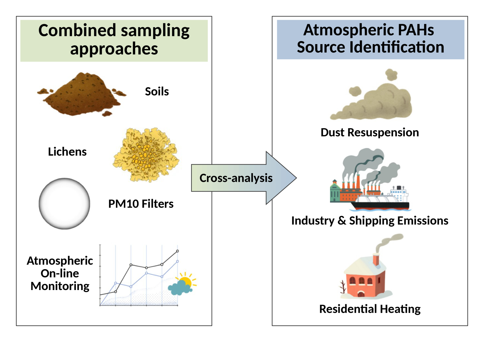
The diversity of PAH sources complicates their identification at receptor sites, and the estimation of their respective contributions, which may in turn delay the implementation of effective mitigation strategies to reduce population and ecosystem exposure. Source identification of atmospheric PAHs can be approached using diagnostic ratios, but that elucidate a limited number of emission sources, generally pyrogenic and petrogenic, and preferably rely on predefined emission profiles (Tobiszewski & Namieśnik, 2012; Harner et al., 2018). These ratios are also subjected to various environmental influences (e.g. reactivity, gas-phase partitioning, particle size, seasonality…) (Shahpoury et al., 2016; Tomaz et al., 2016). More robust source apportionment approaches involving environmental monitoring combined with multivariate analyses (e.g. principal component analysis (PCA), positive matrix factorisation (PMF)…) can provide valuable insights, but their high analytical and logistical costs (e.g. power supply, regular maintenance...), restrict their spatial deployment. In the context of a city-scale exposure to potentially unknown and multiple PAH sources, it becomes necessary to optimize both the efficiency and reliability of source identification to support effective regulatory action. In this context, the present study combines several complementary approaches to determine the major sources contributions to PAH exposure and to gain a broader understanding of PAH transfer and exposure pathways.
To achieve these objectives, an integrated methodology involving soils and atmospheric investigations using both instrumental and biomonitoring techniques, was applied. PAH concentrations in PM10, determined through filter sampling, provided a temporal perspective on atmospheric PAH levels. In parallel, atmospheric biomonitoring using lichens, a well-established method to assess PAH bioaccumulation (Blasco et al., 2006; Nascimbene et al., 2014; Augusto et al., 2015; Dron et al., 2021) was performed to provide spatial data. Lichen bioaccumulation provides a complementary perspective to PM10 filter analyses by integrating exposure over longer timescales (typically several months), reflects interactions with a broader range of particle size, possibly including volatile PAH fractions, and includes biodisponibility aspects. Finally, soils were also investigated, as they may act as both a major source of PAHs through the resuspension of contaminated soil particles (Harner et al., 2018) and a long-term sink via atmospheric deposition (Froger et al., 2021). Therefore, soil PAH contamination reflects long-term cumulative exposure (over several years) and provide an overview of the spatial distribution of contamination, particularly that associated with the deposition of coarse particles, which generally dominate the mass fraction compared to fine particles (Hu et al., 2021). To complete PAH measurements in PM10, lichens and soils, a continuous instrumental monitoring was established for one year, limited to black carbon, SO2 and meteorological data.
Multi-angle approaches have previously been used to elucidate atmospheric contamination, often focusing on an identified activity to assess its impacts on surrounding areas, such as the numerous coordinated projects around the Canadian Athabasca oil sands region (Harner et al., 2018). In contrast, our study applies this approach to a suspected multi-source atmospheric PAHs exposure at the city-scale in the Gulf of Fos area (France), which hosts one of the largest industrial and harbour complexes in Europe. Previous studies have shown that this area is particularly exposed to atmospheric PAHs, likely due to multiple emission sources (Ratier et al., 2018; Austruy et al., 2021). Potential sources include current industrial activities, legacy contamination from soil resuspension, maritime shipping, road traffic, residential heating, and agriculture stubble burning, and possible regional atmospheric inputs.
The aim of this study is to evaluate the capacity of the combined approach (based on analyses in PM10, lichens, and soils) to resolve a complex situation of atmospheric exposure to PAHs. This work seeks to provide a consistent ranking of the main contributing sources and to clarify exposure pathways, with the ultimate goal of improving risk assessment methodologies and supporting environmental management decisions.
Materials and methods
Sampling area
This study focused on Port-Saint-Louis-du-Rhône, a city located in the Gulf of Fos in France. The city covers an area of about 74 km2 and has around 8,600 inhabitants. It is surrounded by a highly contrasted environment, with the large industrial and harbor complex of Fos-sur-Mer to the northeast, the extensive Camargue Regional Nature Reserve to the northwest, and the Mediterranean Sea to the south (Figure 1). Finally, the northern part of the area is influenced by agricultural activities in the Rhône plain, mainly rice and cereal cultivation. The area is subject to multiple atmospheric influences, particularly from industrial emissions from a wide range of activities including refining, petrochemical industry, chemical industry, coke production, steel manufacturing, cement production, and the incineration of household and industrial waste, as well as Style de paragraphe par défautfrom major maritime terminals handling containers, ore, oil, gas and cereals. Previous studies have highlighted the occurrence of numerous contamination events (Austruy et al., 2016, 2019; Sylvestre et al., 2017; Ratier et al., 2018) and documented their environmental (Dron et al., 2019; Lebaron et al., 2019; Austruy et al., 2021) and human health (Jeanjean et al., 2021, 2022) consequences.
The industrialization of Port-Saint-Louis-du-Rhône preceded that of the currently operating industrial facilities. In fact, from the late 19th century until the 1970s, the city experienced significant industrial activity, driven by maritime traffic and its location near the Rhône River mouth. Most factories were located to the south and south-east part of the city. However, the 1974 economic crisis and the development of marine transport led to these activities being transferred to the new industrial harbour of Fos-sur-Mer. The former industrial sites were subsequently abandoned, leaving numerous brownfields sites in the city center and could potentially act as sources of resuspension of contaminated soils. Apart from industrial sources, stubble-burning is widely practiced north of the city in late autumn and winter (rice fields, cane hedges), representing another potential source of airborne contaminants. Common urban sources such as road traffic and residential heating also contribute to local emissions, along with other possible regional unidentified influences. Consequently, the sampling locations (Figure 1) were selected to provide a representative overview of the different expected exposure conditions across the city, encompassing residential zone and potential emission sources from all directions.
The study area has a typical Mediterranean climate, with mean temperatures ranging from 2.9 to 11.4 °C in January and from 19.4 to 30.2 °C in July. Rainfall mainly occurs in autumn and spring, often as heavy episodes, with an annual total of 515.4 mm distributed over an average of 53.2 rainy days (based on the 1981–2010 reference period from the Météo-France data of the Marignane station, 30 km east of the study area (Météo-France, 2020)). The dominant wind direction is from north-northwest (the so-called Mistral, accounting for 40-50% of annual occurrences), often strong and exceeding 100 km.h-1 on several days per year. Other winds include the Marin from the southeast and the Levant from the east. Sea-breeze events are also frequent under stable weather conditions, particularly in summer (Météo-France, 2025; Dron et al., 2021).
It should also be noted that France experienced a full lockdown during part of the study period, lasting 55 days from 17 March to 11 May 2020, in response to the COVID-19 pandemic. While this lockdown clearly affected road traffic and related emissions, industrial and maritime activities in the Fos industrial and harbor complex were not significantly reduced. Atmospheric emissions from residential heating, agriculture, and soils resuspension were likewise unaffected. Still during the study period, a partial lockdown occurred from 30 October to 15 December 2020 (45 days), but it did not result in any notable decrease in traffic or other emission sources (industry, shipping, agriculture, or heating).

Figure 1 – Port-Saint-Louis-du-Rhöne context (left) and location of the sampling sites (right)
Atmospheric on-line monitoring and filter collection
Atmospheric data and PM10 filters were collected at the ambient air monitoring station of the regional Air Quality Monitoring network (Atmosud), located in the city center of Port-Saint-Louis-du-Rhône (near site S3, Figure 1). On-line measurements were continuously recorded throughout the study period (01/01/2020 - 31/12/2020), and include: (i) PM10 concentrations, measured every 15 minutes with a continuous particle monitor (BAM-1020, Met One, USA), (ii) SO2 concentrations measured every 15 minutes using a UV fluorescence analyzer (Model 100E, Envitec, UK), (iii) wind speed and direction measured every minute, (iv) Black Carbon (BC) concentrations in PM2.5, measured every 15 minutes with an aethalometer (AE33-7, Magee scientific, USA), also the BC monitoring allowed differentiation between BC originating from wood burning (BCwb) and BC originating from fossil fuel combustion (Bcff).
Temperature and rainfall data were obtained from a weather station in Fos-sur-Mer, located 12 km northeast of the study area (Figure 1). Weekly data for 2020 are provided in the Appendix A.
The average data availability rates during the study period were: 91.6% for PM10, 92.0% for BC, 78.9% for SO2, 96.0% for wind data and 96.6% for temperature and rainfall.
Quartz fiber filter (150 mm Pallflex® Tissuquartz, pre-baked at 500°C for 5h) were collected every six days, using a high-volume PM10 sampler (Digitel DA80). The device continuously collected air at a flow rate of 30 m3 h-1 for 24 hours. After sampling, filters were retrieved weekly and stored at -40 °C until analysis.
Soil and lichen sampling and preparation
Lichens samples were collected during two campaigns at 7 sites (S1 to 7, Figure 1), on February 26 and June 2, 2020. Soils samples were collected at ten sites (S1 to S10, Figure 1) on March 5 and 11, 2020.
For soil sampling, each site was delineated as a 10 m x 10 m square, from which 9 soils cores were taken: one at the center, one at each corner, and one at the middle of each side (Austruy et al., 2016). Approximately 250 cm3 of surface soil (0-15 cm) were collected with a hand auger and stored at 4 °C. In the laboratory, 100 g of each sample were collected using the quartering method after homogenization and removal of coarse material. The subsamples were combined to form one composite sample per site. The composite samples were lyophilized (-55 °C, 0.035 mbar, Christ Alpha 1-4LD), sieved to 2 mm and stored at -40 °C until analysis. Details of the site-specific soil characteristics are provided in Appendix B.
Lichens were collected according to established protocols (Ratier et al., 2018; Dron et al., 2021). Approximately 10 g (wet weight) of whole Xanthoria parietina thalli were collected using a ceramic knife from 5 to 10 tree trunks at heights between 1.2 to 2 m to avoid soil contamination. Details of the tree species collected at each site are provided in Appendix C. Samples were immediately placed in a Nalgene® flask and stored at 4 °C. Within 24 h, samples were sorted using non-metallic tools (ceramic knife and antistatic plier) to remove dust, bark and other unwanted species.They were then lyophilized (−55 °C, 0.035 mbar, Christ Alpha 1-4LD) and crushed to a fine powder using a crusher equipped with zirconium coated bowls and balls (Retsch MM400 - frequency 25 Hz – 2.5 min). Finally, all samples were stored at −40 °C until analysis.
Chemical analyses
PAHs were analyzed for the 16 congeners from the U.S. EPA priority list : naphthalene (Nap), acenaphthylene (Acy), acenaphthene (Ace), fluorene (Flu), anthracene (Ant), phenanthrene (Phe), fluoranthene (FlA), pyrene (Pyr), benzo(a)anthracene (BaA), chrysene (Chr), benzo(a)pyrene (BaP), benzo(b)fluoranthene (BbF), dibenzo(ah)anthracene (DBA), benzo(k)fluoranthene (BkF), benzo(ghi)perylene (Bpe), and indeno(1,2,3-cd)pyrene (Ipy).
First, an accelerated solvent extraction (ASE 350 Dionex) was carried out, at 100 bar and 100 °C. The solvents used were dichloromethane/acetone (50/50, v/v) for stamped PM10 filters and soils samples, while pure dichloromethane was used for lichens samples. Samples were spiked with anthracene-d10 (Sigma-Aldrich) used as an internal standard prior to extraction. Extracts from all samples were collected, evaporated under a gentle nitrogen stream at 40 °C (TurboVap II, Biotage) and reduced to a volume of 500 µL in hexane. In addition, lichens extracts were purified on a silica cartridge (Supelco Discovery DSC-Si, 6 mL, 1 g, Sigma-Aldrich), and concentrated to a final volume of 500 µL. All samples were finally filtered through a 0.45 µm PTFE syringe filter before analysis. PAHs were quantified using trace gas chromatography coupled to a Quantum XLS mass spectrometer (GC-MS, Thermo Scientific), equipped with a capillary column (TR- 5MS, Thermo Scientific, 30 m x 0,25 mm x 0,25 µm). Helium was used as carrier gas at a constant flow rate of 1 mL.min-1. 1 μL of the sample was injected in splitless mode at 280 °C. The GC oven temperature program was as follows, initial temperature 65 °C (held for 1 min), ramped to 300 °C at a rate of 6 °C.min-1 and held at 300°C for 20 min. The ion source temperature was fixed at 250 °C and the mass spectrometer operated in the electron impact ionization mode (70 eV), alternately in Full Scan mode (m/z 45 –500) and in Single Ion Monitoring (SIM) mode to target specific ion fragments of each PAH compound for quantification. Data processing was carried out using the Thermo Scientific Xcalibur software.
The results of the quality controls by the analysis of certified materials (IAEA-383 and IAEA-451) are given in the appendices (Appendix D). The certified materials were prepared and analysed in the same way as the soil (IAEA-383) and lichen samples (IAEA-451). All IAEA-383 measurements fell within the 95% confidence interval, and all IAEA-451 measurements fell within the ± 20% target range, with the exception of DBA.
Data analysis
Statistical analyses were performed using R software (version 3.5.2) (R Core Team, 2016), and visualizations were enhanced using the vector graphics editor Inkscape. For statistical treatment, compounds that were below the detection limit detected (nd) were considered as zero, and below the limit of quantification (<l.q.) were assigned a value of ¼ of that limit. To compare PAH profiles between sites, Spearman’s rank correlation coefficients was calculated, as the Shapiro normality test indicated deviations from normality (Appendix F). This non-parametric approach is suitable for small and independent sample sets (one replicate per sample type). These coefficients (ρ) were calculated based on the relative level of each PAH concentration in relation to the total PAH concentration (Σ16PAH) (expressed as a percentage) in order to focus on relative distributions that may reflect specific signatures rather than total concentration levels. Atmospheric data were analyzed using the R package “openair” (Carslaw & Ropkins, 2012). A Multiple Correspondence Analysis (MCA) was performed to explore associations among qualitative variables and the predominant wind typologies observed in the study area (north, south-east, sea breeze, and other). Finally, maps were created using the QGIS 3.8 software.
Results
PAHs in soils

Figure 2 - Σ16PAH concentrations measured in soils from 10 sampling sites
The total concentrations of the 16 priority PAHs (Σ16PAH) measured in surface soil samples in winter are presented in Figure 2. All soil samples contained measurable levels of PAHs, but concentrations measured were highly heterogeneous ranging from 402 µg.kg-1 (S2) to 30 747 µg.kg-1 (S1). For comparison, PAH concentrations usually observed in typical French soils generally range between 100 and 1 000 µg.kg-1 (Bour, 2005). These results revealed significant soil contamination at several sites, particularly S1, located on a brownfield site with known historical PAH contamination, but also S5 and S9, where Σ16PAH exceeded 10 000 µg.kg-1. Intermediate concentrations were observed at S3, S8, and S6 (2 700-3 300 µg.kg-1). Thus, the spatial distribution revealed a decreasing gradient in PAH concentrations from S1 towards the north-northwest and southeast.
Detailed concentrations of each of the 16 PAHs are given in Appendix E. Overall, the distribution of PAHs was similar across the samples, with a predominance of high-molecular-weight PAHs (HMW PAHs) containing 4 to 6 aromatic rings, commonly associated with aged or historical soil contamination. This distribution may result from the preferential depletion of low-molecular-weight PAHs (LMW PAHs) with time through processes such as leaching, evaporation, volatilization and biodegradation, to which LMW PAHs are generally more susceptible because of their higher volatility and greater susceptibility to microbial degradation (Wilcke, 2000; Gundlapalli et al., 2024). However, the rates of these processes are also influenced by soil propreties, particularly organic matter content and texture. In soils with higher organic matter contents, the depletion of LMW PAHs through volatilization and biodegradation may be delayed because of stronger sorption to the soil matrix. In the present study, the sampling soils had sandy-loam textures, while organic matter contents ranged from 1.3 to 8.2 % (Appendix B). These differences in soils propreties may have contributed to variations in PAH retention and degradation among sites, the predominance of HMW PAHs likely reflects a combination of post-depositional weathering processes and site-specific soil characteristics.
These distribution patterns are supported by Spearman’s correlation tests and associated p-values (Appendix G), which helped identify relationships between soil PAH profiles. The most contaminated site, (S1 a brownfield area), showed the highest similarity with S5, S8 and S9 (ρ ranged between 0.90 and 0.92, p<0.05), all located in the city center, indicating that the PAH distributions in these sites are comparable. Strong correlations were also observed within these sites (S5, S8 and S9) themselves (ρ ranged between 0.96 and 0.98, p<0.05). In contrast, weaker correlations were found between S1 and S2 (ρ=0.54, p<0.05) and between S1 and S7 (ρ=0.62, p<0.05), both northern sites. Site S3, which is also located in the city center, correlated with S4 and S10 (both ρ=0.95, p<0.05), both situated in the eastern coastal part of the city near the industrial harbour. These two sites were also strongly correlated with each other (ρ=0.97, p<0.05) and were characterized by a higher proportion of LMW PAHs (2-3 rings), suggesting more recent atmospheric inputs, potentially linked to industrial emissions from the harbour area (Hubai et al., 2025). Finally, the northernmost sites, S2 and S7, showed limited similarity with the other sites (ρ ranged between 0.63 and 0.75, p<0.05), except for a moderate correlation between S7 with both S4 and S10, consistent with its higher proportion of LMW PAHs.
Bioaccumulation in lichens
The Σ16PAH concentrations measured in the lichen samples are presented in Figure 3. The results indicate a continuous exposure to PAHs across both sampling periods, with consistently higher bioaccumulation levels in winter. Concentrations were highly variable, ranging between 222 µg.kg-1 (S2) and 2459 µg.kg-1 (S1) in winter (February 2020), and between 173 µg.kg-1 (S2) and 1363 µg.kg-1 (S1) in summer (June 2020). Using the same lichen biomonitoring methodology, Dron et al. (2016) reported total PAH levels between 237 and 620 µg.kg-1 in lichen samples collected in cities near the Fos-sur-Mer industrial harbour except, as previously mentioned, in Port-Saint-Louis-du-Rhône where higher concentrations were measured (1 165 to 2 034 µg.kg-1). In the present study, PAH levels were overall elevated and exceeded those reported in other European industrial regions, such as Sines (Portugal, 249 µg.kg-1, Augusto et al., 2010), Manchester (UK, 189.8 µg.kg-1, Niepsch et al., 2024), and Tarragona County (Spain, 480.0 µg.kg-1, Domínguez-Morueco et al., 2017).
As for the soils, the spatial distribution of lichen contamination showed a gradient of decreasing concentrations from S1. Site S1 exhibited the highest PAH contamination levels (1363-2459 µg.kg-1), followed by S5, located nearby. The lowest concentrations were measured at S2 and S7, in the northern part of the city. The levels recorded at these two sites were comparable to those observed in rural locations during previous lichen biomonitoring campaigns in the region (Dron et al., 2016; 2021; Ratier et al., 2018), and can thus be considered representative of local PAH background levels in lichens.
Detailed concentrations of the 16 PAHs individual measured in each sample are provided in Appendix E. As in soils, lichen PAH profiles were dominated by HMW compounds (4-5 rings PAHs). Some seasonal variations were observed, with most sites showing higher proportions of 3 rings PAHs in summer, and higher proportions of 5-rings PAHs in winter, while 4-rings PAHs proportions remained stable across seasons. Sites S1 and S5 exhibited limited seasonal variation in PAH distributions, suggesting stable sources throughout the year. In contrast, other sites showed more pronounced seasonal variations in PAH profiles, indicating variable influences depending on atmospheric conditions. Additionally, S4, S6 and S7 had a higher proportion of LMW PAHs (2 and 3-rings PAHs) than the others, supporting the hypothesis of distinct or more recent emission sources at these locations, consistent with previous observations in soils for S4 and S7.

Figure 3 - Σ16PAH concentrations measured in lichens from 7 sampling sites
The Spearman’s correlation tests were performed (Appendix H), to identify samples with similar PAH distributions patterns and to assess potential seasonal variations. Overall, correlations were stronger in February than in June 2020, indicating more homogeneous PAH distributions among sites during winter. This suggests a more uniform atmospheric influence on PAH signatures in that period.
Consistent with the soil results, the correlation coefficients calculated for lichens reflected the spatial gradient in total PAH concentrations, allowing direct comparisons between soil and lichen contamination patterns. A strong correlation was observed between S1 and S5 in both seasons (ρ=0.96-0.98, p<0.05), but these two sites showed limited similarity with the others. Site S2 displayed generally weak correlations with most sites, except with S4 in both winter and summer (ρ=0.90-0.96, p<0.05), and with S7 in summer (ρ=0.98, p<0.05), suggesting distinct source influences. As expected, S4 and S7 were also correlated, particularly in summer (ρ=0.94, p<0.05). The remaining sites, S3 and S6, were strongly correlated in winter (ρ=0.96, p<0.05).
Atmospheric on-line monitoring
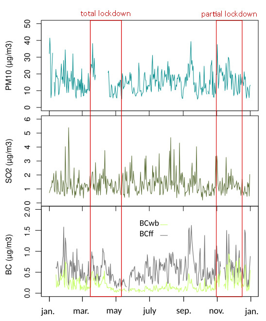
Figure 4 - Average daily concentrations of PM10, SO2 and BC measured at the atmospheric station of AtmoSud from 01/01/2020 to 31/12/2020
Figure 4 shows the evolution of the daily average concentrations of PM10, Black Carbon (BC) and SO2 (in µg.m-3) calculated from the quarter-hourly data collected between January 1 and December 31, 2020.
Based on the quarter-hourly dataset, the annual average concentrations and corresponding ranges of values for the various variables were as follows: 15.4 µg.m-3 [0.1-153.9 µg.m-3],
1.4 µg.m-3 [0.0-48.2 µg.m-3], 0.6 µg.m-3 [0.0-14.9 µg.m-3] and 0.2 µg.m-3 [0.0-4.2 µg.m-3] for PM10, SO2, BCff and Bcwb, respectively. As shown in Figure 4 neither the full COVID-19 lockdown (17 March – 11 May) nor the partial lockdown (30 October – 15 December) had a marked effect on these parameters in the study site.
Furthermore, important variations were still observed. The evolution of total BC levels showed globally higher levels in winter, with averages concentration of 0.9 µg.m-3 in December-February compared to 0.7 µg.m-3 in June-August, and frequent daily peaks during the cold season. Throughout the year, BCff contributed more to total BC than BCwb. However, BCwb exhibited strong seasonal variability, with significantly higher levels in winter and autumn, reflecting increased biomass burning for domestic heating during the cold season. In contrast, these PM10 and SO2 concentrations remained relatively stable throughout the year, showing no clear seasonal trend.
PAH levels in PM10

Figure 5 - Variations of total PAH concentrations in PM10 and PM10 concentrations (24h period every 6 days) measured from 07/01/2020 to 31/12/2020 at the atmospheric station of AtmoSud
During one year, Σ16PAH concentrations was measured in PM10 filter samples to assess the contribution of PM10 in the inputs of PAHs (Appendix I). Figure 5 shows the evolutions of PAH concentrations in PM10 together with the corresponding daily PM10 averages. The annual mean concentration of PAHs in PM10 at Port-Saint-Louis-du-Rhône (1.95 ng.m-3) was comparable to or higher than those reported for major European cities (1.0-2.1 ng.m-3) by Jedynska et al. (2014), the highest levels in that study being observed in Copenhagen and Rome (2.1 and 2.0 ng.m-3, respectively). Our mean annual PAHs concentration was also higher than that reported by Varea et al. (2011), in Alicante (Spain), at a coastal urban site near a cement plant (1.15 ng.m-3).
The PAH profiles were dominated by 5-rings PAHs, followed by 4-rings compounds, with seasonal variations observed. The relative abundance of 5-rings PAHs was higher in winter (Dec-Jan-Feb: 52.2%) than in summer (Jun-Jul-Aug: 39.1%), whereas 3-rings PAHs were more abundant in summer (14.3%) than in winter (4.2%). The proportions of 4- and 6-rings PAHs remained stable between these periods. The trends are consistent with the observations made in lichens. In addition, PAH concentrations in PM10 were markedly higher during autumn and winter, with a maximum concentration of 19.6 ng.m-3 recorded on 11 November 2020. This suggests that residential heating was a substantial contributor to atmospheric PAHs in PM10, potentially amplified by thermal inversions events typical of winter. The higher winter contribution of residential heating was further supported by the increase in BCwb levels during this period, while BCff remained relatively stable, and was consistent with the higher PAH concentrations measured in lichens in late winter (Feb. 2020).
The congener benzo(a)pyrene (BaP) is commonly used as an indicator of carcinogenic PAHs (WHO, 2000) and several countries have established air quality standards for this compound. In the European Union, a target value of 1.0 ng m-3 expressed an annual average in PM10 was established (Directive 2004/107/EC) (European Parliament and Council, 2004) and subsequently adopted in French legislation. By comparison, the annual average calculated from the 66 PM10 filters analyzed in this study for 2020 was 0.16 ng.m-3.
However, particulate PAHs are generally not uniformly distributed across the aerosol size fractions. They preferentially associate with the fine fraction (PM2,5) rather than with the coarse fraction (PM10), and this tendency is even more pronounced for HMW compounds (Albagli et al., 1974; Ravindra et al., 2008; Zhang et al., 2020). Several studies have investiged the distribution of PAHs between the fine and coarse fractions. For example, Varea et al. (2011) reported that around 80 % of total PAHs were associated with the fine fraction (PM2.5) and 20 % in the coarse one (PM2.5-10), corresponding to PM2.5/PM10 ratios ranging from 0.75 to 0.87. More specifically, for benzo(a)pyrene, Siudek & Ruczyńska (2021) reported an average PM2.5/PM10 ratio of 0.70 ± 0.23 at a coastal urban site influenced by industrial emissions similar to those in the present study. In the absence of measure of PAHs in PM2,5, published PM2.5/PM10 ratios provide a useful basis for estimating PAH concentrations in the fine fraction from PM10 measurements. Nevertheless, these Météo-France ratios should be regarded as indicative only, as they may vary considerably depending on emissions sources, meteorological conditions, and spatial and seasonal variability.
Discussion
These results, obtained from the different environmental monitoring approaches, highlighted the city’s specific and complex context, characterized by multi-source, and diffuse PAH contamination. Those compounds were ubiquitous across all sample types at high concentrations.
To further identify the origins of PAHs measured in PM10, on-line atmospheric data measured during the sampling days of the filters (PM10, BCff, BCwb, SO2, wind direction and speed) were integrated with the Σ16PAH concentrations in PM10 using a Multiple Correspondence Analysis (MCA) (Figure 6). The results will subsequently be combined with lichen and soil data to help determine the dominant PAH sources influencing the study area.

Figure 6 - Multiple Correspondence Analysis (MCA, principal components PC1 and PC2) realized on atmospheric data, Σ16PAH concentrations in PM10 and wind conditions (n = 60)
These results highlighted the mixed influence of industrial emissions and residential heating on environmental exposure. The first two axes (PC1 and PC2) of the MCA explained 65.5% of the total variance. The first component (PC1), accounting for 42.0% of the variance, was characterized by a strong association between the variables SO2, PM10, PAHs in PM10, BCff and BCwb under southeasterly and sea breeze wind conditions and anti-correlated with the wind speed and north wind conditions. This supports the hypothesis that most PAHs in PM10 originated from the industrial harbour area, as maritime transport and industrial emissions are major sources of SO2, while the association with BCwb, also indicates contributions from biomass burning (residential heating and agriculture). The implication of current industrial activities and maritime transport was further supported by the second axis (PC2), which accounted for 23.5% of the variance, and maintained the associated between SO2, PM10 and PAHs in PM10.
The identification and ranking of PAH sources are discussed and evaluated by type of emissions.
Dust resuspension from brownfields
The city-center of the study area contains numerous brownfields site, a large part situated between S1, S4, S5 and S10. However, wind-driven erosion of contaminated soils likely results in the resuspension of dust containing high levels of PAHs (Young et al., 2002; Tian et al., 2021; Ejileugha & Otu, 2025). Site S1, located on one of these brownfields, historically involved in oil transformation and storage, showed the highest soil PAH concentrations. Despite the weak soil mobility of PAHs, a decreasing concentration gradient starting from site S1 was visible on the soil’s contamination mapping, starting from site S1 (Rollin et al., 2005). A similar gradient was also observed in lichen bioaccumulation results. Thus, the resuspension of dust from brownfield sites is supported by lichen and soil gradients centered around these wastelands. Lichen data further suggested that this contribution is more important than seasonal emissions (residential heating, agricultural burning) since the spatial gradients were more pronounced than seasonal variations. This interpretation was reinforced by statistical analysis showing strong similarities of PAH distribution between S1 and S5 in lichens, and among S1, S5, S8 and S9 in soils. Additionally, the absence of significant seasonal variation in lichen PAH profiles at S1 and S5, implying a similar origin in time and indicated a persistent, local emission source. The consistency between soil and lichen gradients and congener distributions suggests that both matrices reflect comparable PAH exposure patterns, i.e. coarse particles from contaminated soil resuspension.
In summary, the spatial and compositional similarities between soils and lichens suggesting that contaminated soils dust resuspension may be an important PAH pollution source across inhabited areas, in particularly through coarse particles.
Also, during the study, deposition gauges (Owen gauges) were installed at sites 1, 2 and 3 during the winter (17 December 2019 to 15 January 2020). The methodology and data obtained were included in Appendix J. The results support these interpretations, showing greater dust levels and higher PAHs deposition at S1 compared to S2 and S3. Additional data would help to consolidate these observations.
Industrial and shipping emissions
Sites S4 and S10 are expected to reflect the influence of ongoing industrial activities through their location away from the urban center but closer and downwind of the industrial-port area and maritime traffic. This assumption is supported by the higher proportions of LMW PAHs in soil and lichen samples from these sites, characteristic from recent emissions (Wu et al., 2006). Significant similarities were also observed between the PAH congener distribution of the soils from the urban site S3 and those from S4 and S10, suggesting that current industrial emissions likely affect the entire urban area.
According to the MCA results atmospheric PAH concentrations near to the atmospheric station were closely correlated with SO2 and PM10, and associated with southeasterly and sea breeze conditions. Under these wind patterns, the city is exposed to emissions from marine traffic and industrial zones of from Martigues-Lavera and the industrial-port complex of Fos-sur-Mer, which include major PAH-emitting facilities such as refineries, petrochemical plants, coke production, and steel industry (El Haddad et al., 2009; Sylvestre et al., 2017). This suggests a significant contribution of current industrial activities to the presence of PAHs in atmospheric particulate matter.
Previous studies (Dron et al., 2016; Ratier et al., 2018) showed that lichen contaminant concentrations, including PAHs, increase markedly near industrial areas. Elevated PAH levels were reported in cities near the industrial-port area of Fos-sur-Mer, confirming its local influence on atmospheric contamination. However, the even higher PAH levels observed in Port-Saint-Louis-du-Rhône suggest that industrial emissions, although important for PM10-bound PAHs, may not be the sole contributors to total environmental PAH burdens, consistent with the potential role of resuspended soils.
Therefore, current industrial emissions appear to be the main contributors to PAHs in PM10, but not to the overall PAH load in coarse particles, as indicated by lichen and soil data. However, despite their smaller mass contribution, fine particles are of particular concern for human health because of their deeper penetration into the respiratory system.
Residential heating
Seasonal variations were observed in both lichens and atmospheric PM10, with higher PAH concentrations and higher proportions of HMW PAHs during winter. Additionally, BCwb levels were higher in winter than in summer, reflecting emissions from residential wood burning for heating, whereas SO2 and PM10 did not exhibit significant seasonal variability. This is consistent with the literature (Jedynska et al., 2014). Nevertheless, in lichens, the seasonal increase in PAH content was smaller than the spatial increase observed near brownfield sites, indicating that resuspended soil contamination remained the dominant source.
Meteorological conditions also play a key role. Colder temperatures and cloudy conditions can enhance PAH levels by reducing degradation rates, reducing the boundary layer height and inducing thermal inversion (Qiu et al., 2013; LCSQA, 2003). Under such conditions, gas-particle phase partitioning shifts toward the particulate phase, particularly for LMW PAHs (Ravindra et al., 2008). Although these processes promote higher PAH concentrations in winter, biomass burning for residential heating remains a significant source, especially for PAHs in PM10, and to a lesser extent, for larger particle reflected in lichens.
Other seasonal phenomena may have had a impact on our results. Weekly weather data (Appendix A) indicate that precipitation was almost negligible the weeks before the winter campain, whereas rainfall records from the neighby Istres monitoring station (used as a proxy because local data were unavailable) indicate wetter conditions prior to the summer campaign. This contrast may have influenced the results, as precipitation can reduce dust resuspension by increasing soil moisture. Rainfall may also have a ‘wash-off’ effect on contaminants accumulated on the lichen thalli (Root et al., 2021; Niepsch et al., 2024).
Also during the summer campaign, the tree canopy may also have influenced contaminant deposition. Depending on its presence and density, it could have acted as a physical barrier, intercepting airborne particules before they reached the lichen thalli. Because canopy cover differed among the sampling sites, this interception effect may have varied spatially. In fact, phorophytes differed among sites and season (Appendix C) and substrates where lichens are collected from may influence pollutant accumulation (Augusto et al., 2013). However, Dron et al. (2021) reported that the influence of these factors was minor in the study area.
Agricultural stubble-burning
Site S2, and to a lesser extent S7, were located within agricultural areas dominated by rice cultivation, where stubble-burning occurs in winter (typically November to January). In S2, lichen PAH distribution showed clear seasonal variations, with a higher proportion of 3-rings PAHs in summer (32 % in summer vs. 23 % in winter) and 5-rings PAHs in winter (31 % in winter vs. 18 % in summer) while 4-rings PAHs remained the most abundant, in proportions independent of the seasons (38 %). These results suggest a predominantly pyrogenic origin from biomass combustion in this site, located far from residential, brownfields and industrial influences (Chen & Chen, 2011).
These localized effects were not detected across the rest of the city, and PAH distributions in soils and lichens at these sites exhibited the lowest correlation coefficients with urban profiles, confirming distinct origins. Moreover, Σ16PAH concentrations at S2 and S7 were the lowest across all matrices, indicating that agricultural burning exerted only a minor, localized influence, without significant impact on the elevated PAH levels observed elsewhere in the study area.
Conclusion
This study demonstrated the relevance and complementarity of multiple analytical approaches for identifying and ranking PAH sources. The consistency of results across methods highlighted the main contributors to the elevated atmospheric PAH concentrations observed at the city scale, within a complex environment influenced by both historical and current industrial activities.
The combined use of different sampling and monitoring strategies allowed for a comprehensive understanding of environmental exposure that could not have been achieved by any single method alone. Diffuse contamination was identified across environmental matrices, with high average PAH concentrations in the lichens and soils, which seem primarily driven by resuspension of contaminated soil particles. Industrial emissions from the nearby industrial-port complex also contributed to PAH levels, establishing an urban background comparable to that of other cities in the Gulf of Fos area. Strong seasonal variations were observed in all datasets, with higher concentrations in winter, mainly attributable to domestic heating, while agricultural burning played a limited role. The spatial mapping of soils contamination provided an initial identification of the most exposed areas, particularly brownfields and the city center, indicating substantial exposure risks for the local population.
The COVID-19 lockdown periods did not significantly affect PAH levels in PM10, neither the other on-line atmospheric pollutants measured, suggesting that non-commercial road traffic contributed only marginally to PAH concentrations in this area.
Discussions with local authorities have been held to explore the vegetation of brownfield sites as a strategy to limit contaminated soil resuspension and reduce atmospheric PAH exposure, which constitutes a significant public health concern given the high cumulative exposures reflected by elevated levels in samples.
Acknowledgements
All authors are thankful to the SUD-PACA Regional Directorate for the Environment Development and Housing, through the Health and Environment Regional Program (PRSE), for financial support. Authors are also grateful to the city of Port-Saint-Louis-du-Rhône, Marseille-Fos Port authorities, Mrs Carle, the “Citron Jaune” artists association, Mr Monturli, and Mr Guedj for access to landfills and other sites.
We also thank the reviewers for helpful comments on a previous version of this paper. Preprint version 3 of this article has been peer-reviewed and recommended by Peer Community In Ecotoxicology and Environmental Chemistry (https://doi.org/10.24072/pci.ecotoxenvchem.100452; Gagnon, 2026).
Funding
Annabelle Austruy reports financial support was provided by Regional Directorate for the Environment Development and Housing for this work.
Conflict of interest disclosure
The authors declare that they comply with the PCI rule of having no financial conflicts of interest in relation to the content of the article.
Data, scripts, code, and supplementary information availability
Data to reproduce all analyses presented in this paper are available in appendices (lichen, soil data and meteorology) and from Atmosud website atmosud.org (PM10, SO2, black carbon).
Appendixes
Appendix A – Meteorological conditions
|
Week |
Period |
Rain accumulation (mm) |
Mean temperature [Min – Max] (°C) |
NA (day) |
|
1 |
30/12/2019 - 05/01/2020 |
0.00 |
8.30 [0.80 – 14.1] |
5 |
|
2 |
06/01 - 12/01/2020 |
2.60 |
8.40 [1.10 – 16.0] |
- |
|
3 |
13/01 - 19/01/2020 |
6.70 |
9.10 [0.50 – 15.0] |
- |
|
4 |
20/01 - 26/01/2020 |
34.1 |
10.3 [4.00 – 16.1] |
- |
|
5 |
27/01 - 02/02/2020 |
19.4 |
10.7 [3.00 – 19.0] |
- |
|
6 |
03/02 - 09/02/2020 |
0.70 |
10.8 [4.30 – 21.3] |
- |
|
7 |
10/02 - 16/02/2020 |
0.00 |
11.4 [3.30 – 18.6] |
- |
|
8 |
17/02 - 23/02/2020 |
0.00 |
10.7 [3.30 – 19.0] |
- |
|
9 |
24/02 - 01/03/2020 |
3.90 |
11.1 [2.50 – 23.4] |
- |
|
10 |
02/03 - 08/03/2020 |
4.40 |
10.2 [2.90 – 15.8] |
- |
|
11 |
09/03 - 15/03/2020 |
0.30 |
13.0 [6.60 – 23.5] |
- |
|
12 |
16/03 - 22/03/2020 |
0.00 |
12.7 [5.60 – 19.4] |
- |
|
13 |
23/03 - 29/03/2020 |
4.20 |
10.0 [0.80 – 19.7] |
- |
|
14 |
30/03 - 05/04/2020 |
0.00 |
11.1 [4.70 – 18.7] |
- |
|
15 |
06/04 - 12/04/2020 |
0.00 |
13.9 [5.40 – 23.6] |
- |
|
16 |
13/04 - 19/04/2020 |
1.20 |
15.0 [8.60 – 24.0] |
- |
|
17 |
20/04 - 26/04/2020 |
4.10 |
15.7 [11.0 – 21.9] |
- |
|
18 |
27/04 - 03/05/2020 |
43.6 |
17.6 [10.6 – 26.1] |
- |
|
19 |
04/05 - 10/05/2020 |
11.8 |
18.2 [11.7 – 26.6] |
- |
|
20 |
11/05 - 17/05/2020 |
NA (Istres : 43 mm)* |
NA |
7 |
|
21 |
18/05 - 24/05/2020 |
NA (Istres : 0 mm)* |
NA |
7 |
|
22 |
25/05 - 31/05/2020 |
NA (Istres : 0,2 mm)* |
NA |
7 |
|
23 |
01/06 - 07/06/2020 |
21.5 |
19.8 [14.4 – 24.6] |
- |
|
24 |
08/06 - 14/06/2020 |
8.90 |
19.3 [13.5 – 27.3] |
- |
|
25 |
15/06 - 21/06/2020 |
0.10 |
21.7 [14.8 - 30.2] |
- |
|
26 |
22/06 - 28/06/2020 |
0.00 |
23.5 [17.2 – 30.4] |
- |
|
27 |
29/06 - 05/07/2020 |
9.40 |
25.1 [18.3 – 34.6] |
- |
|
28 |
06/07 - 12/07/2020 |
0.20 |
24.2 [16.4 – 31.3] |
- |
|
29 |
13/07 - 19/07/2020 |
0.20 |
24.6 [17.6 – 31.4] |
2 |
|
30 |
20/07 - 26/07/2020 |
0.20 |
26.6 [19.9 – 34.7] |
4 |
|
31 |
27/07 - 02/08/2020 |
0.00 |
26.4 [20.1 – 38.7] |
6 |
|
32 |
03/08 - 09/08/2020 |
0.20 |
23.3 [15.6 – 30.4] |
- |
|
33 |
10/08 - 16/08/2020 |
0.00 |
25.4 [19.2 – 32.9] |
- |
|
34 |
17/08 - 23/08/2020 |
0.20 |
25.4 [18.6 – 33.6] |
- |
|
35 |
24/08 - 30/08/2020 |
5.10 |
22.8 [15.2 – 32.7] |
- |
|
36 |
31/08 - 06/09/2020 |
0.20 |
21.2 [14.0 – 29.1] |
- |
|
37 |
07/09 - 13/09/2020 |
24.6 |
22.1 [16.4 – 31.2] |
- |
|
38 |
14/09 - 20/09/2020 |
21.9 |
23.3 [18.1 – 30.3] |
6 |
|
39 |
21/09 - 27/09/2020 |
27.8 |
17.8 [9.40 – 26.3] |
- |
|
40 |
28/09 - 04/10/2020 |
8.90 |
15.4 [8.60 – 22.6] |
- |
|
41 |
05/10 - 11/10/2020 |
1.60 |
15.5 [9.00 – 24.3] |
- |
|
42 |
12/10 - 18/10/2020 |
2.00 |
12.4 [5.90 – 19.0] |
- |
|
43 |
19/10 - 25/10/2020 |
1.90 |
17.0 [6.60 – 21.4] |
- |
|
44 |
26/10 - 01/11/2020 |
0.20 |
14.3 [7.50 – 22.6] |
- |
|
45 |
02/11 - 08/11/2020 |
19.4 |
14.7 [8.90 – 21.5] |
- |
|
46 |
09/11 - 15/11/2020 |
18.5 |
15.0 [8.80 – 20.0] |
- |
|
47 |
16/11 - 22/11/2020 |
11.5 |
10.7 [2.80 – 20.4] |
- |
|
48 |
23/11 - 29/11/2020 |
0.60 |
11.1 [3.20 – 17.9] |
- |
|
49 |
30/11 - 06/12/2020 |
4.60 |
6.30 [-0.20 – 13.9] |
- |
|
50 |
07/12 - 13/12/2020 |
17.2 |
6.50 [0.30 – 13.7] |
- |
|
51 |
14/12 - 20/12/2020 |
6.00 |
12.6 [3.00 – 16.3] |
- |
|
52 |
21/12 - 27/12/2020 |
14.3 |
8.50 [-1.90 – 15.4] |
- |
|
53 |
28/12/2020 – 03/01/2021 |
1.40 |
6.60 [-0.50 – 11.8] |
4 |
*Weather data for the period from 11 to 31 May were unavailable at this station so rainfall data from the neighbouring town of Istres were added as a proxy
Appendix B – Soil properties
|
pH |
Organic matter (%) |
Organic carbon (%) |
Total nitrogen (g/kg) |
C/N ratio |
CEC (me/100g) |
Na2O (g/kg) |
|
|
S1 |
8.3 |
4.0 |
2.3 |
0.79 |
29.5 |
0.4 |
0.02 |
|
S2 |
8.6 |
2.6 |
1.5 |
1.72 |
8.80 |
3.1 |
0.57 |
|
S3 |
8.0 |
4.2 |
2.5 |
2.22 |
11.1 |
4.7 |
0.11 |
|
S4 |
7.9 |
4.3 |
2.5 |
1.66 |
14.9 |
3.3 |
0.04 |
|
S5 |
8.7 |
1.3 |
0.7 |
0.69 |
10.6 |
1.3 |
0.30 |
|
S6 |
9.0 |
2.2 |
1.3 |
1.26 |
10.1 |
8.3 |
3.53 |
|
S7 |
8.2 |
5.0 |
2.9 |
2.92 |
10.0 |
9.1 |
0.34 |
|
S8 |
7.9 |
5.8 |
3.4 |
3.36 |
10.1 |
8.2 |
0.04 |
|
S9 |
7.8 |
8.2 |
4.8 |
3.17 |
15.0 |
5.9 |
0.09 |
|
S10 |
8.2 |
2.6 |
1.5 |
1.41 |
10.8 |
3.8 |
0.04 |
Appendix C – Details of lichen host trees
|
February 2020 |
June 2020 |
|
|
S1 |
7 Morus sp. |
9 Morus sp. |
|
S2 |
3 Fraxinus sp. |
1 Prunus sp. 4 Fraxinus sp. |
|
S3 |
5 Tamarix sp. |
3 Populus sp. 4 Tamarix sp. |
|
S4 |
1 Populus sp. 7 Tamarix sp. |
4 Populus sp. 5 Tamarix sp. |
|
S5 |
7 Tamarix sp. |
9 Tamarix sp. |
|
S6 |
6 Tamarix sp. |
6 Tamarix sp. |
|
S7 |
1 Ficus sp. 3 Tamarix sp. 1 Quercus sp. |
7 Tamarix sp. |
Appendix D – Certified reference material
|
IAEA-451 (Lichens ref.) |
IAEA-383 (Soils ref.) |
|||||||
|
Measured values (n=2) (µg/kg) |
Recommen-ded values (µg/kg) |
Recovery ranges (%) |
Measured values (n=4) (µg/kg) |
Recomme-ded values (µg/kg) |
95% confidence interval (µg/kg) |
Recovery ranges (%) |
||
|
Nap |
12.10 |
14.8 ± 1.2 |
82 |
77.44 |
96 |
52 - 110 |
81 |
|
|
Acy |
18.15 |
- |
- |
33.98 |
47 |
31 - 59 |
72 |
|
|
Ace |
4.03 |
- |
- |
23.92 |
16 |
13 - 21 |
150 |
|
|
Fle |
6.05 |
- |
- |
35.00 |
27 |
24 - 34 |
130 |
|
|
Phe |
23.19 |
15.8 ± 5.6 |
147 |
166.32 |
160 |
140 - 190 |
104 |
|
|
Ant |
15.12 |
- |
- |
29.57 |
30 |
25 - 34 |
99 |
|
|
FlA |
49.40 |
49.3 ± 3.2 |
100 |
323.59 |
290 |
260 - 350 |
112 |
|
|
Pyr |
46.37 |
40.0 ± 4.6 |
116 |
327.73 |
280 |
210 - 350 |
115 |
|
|
BaA |
25.20 |
19.2 ± 1.3 |
131 |
120.06 |
105 |
83 - 130 |
114 |
|
|
Chr |
28.23 |
26.9 ± 2.0 |
105 |
157.03 |
170 |
120 - 220 |
92 |
|
|
BbF |
38.31 |
35.8 ± 6.2 |
107 |
113.91 |
150 |
96 - 190 |
76 |
|
|
BkF |
16.13 |
14.7 ± 3.2 |
110 |
62.64 |
73 |
48 - 76 |
86 |
|
|
BaP |
22.18 |
18.2 ± 2.4 |
122 |
106.70 |
120 |
77 - 140 |
89 |
|
|
DBA |
12.10 |
5.3 ± 1.4 |
228 |
36.62 |
- |
- |
- |
|
|
Bpe |
24.19 |
19.5 ± 2.4 |
124 |
177.48 |
190 |
69 - 230 |
93 |
|
|
Ipy |
29.2 |
- |
- |
147.10 |
- |
- |
- |
|
Appendix E – Details of PAH concentrations in lichen and soil samples
|
[HAP] (µg/kg) |
Lichens (february) |
Lichens (june) |
Soils |
||||||||||||||||||||||
|
S1 |
S2 |
S3 |
S4 |
S5 |
S6 |
S7 |
S1 |
S2 |
S3 |
S4 |
S5 |
S6 |
S7 |
S1 |
S2 |
S3 |
S4 |
S5 |
S6 |
S7 |
S8 |
S9 |
S10 |
||
|
Nap |
7.62 |
0.05 |
4.26 |
14.93 |
11.27 |
25.77 |
41.59 |
14.48 |
5.07 |
24.49 |
6.77 |
8.13 |
13.98 |
7.33 |
309.13 |
0.33 |
20.08 |
9.61 |
22.16 |
26.57 |
11.48 |
2.83 |
58.29 |
15.67 |
|
|
Acy |
15.39 |
1.88 |
3.33 |
3.98 |
4.44 |
3.44 |
5.23 |
14.77 |
8.62 |
11.72 |
10.42 |
9.57 |
9.32 |
8.25 |
204.46 |
0.30 |
2.96 |
4.31 |
4.16 |
3.72 |
2.54 |
1.74 |
22.44 |
2.02 |
|
|
Ace |
2.59 |
0.05 |
2.62 |
1.00 |
6.46 |
2.29 |
0.05 |
6.71 |
2.03 |
5.35 |
4.69 |
7.18 |
3.73 |
2.75 |
37.44 |
0.05 |
24.46 |
3.23 |
42.88 |
10.71 |
3.25 |
8.89 |
50.48 |
10.31 |
|
|
Fle |
14.11 |
3.42 |
8.80 |
10.95 |
18.48 |
8.46 |
8.56 |
15.54 |
5.58 |
12.95 |
9.38 |
14.35 |
7.92 |
5.04 |
29.24 |
0.13 |
18.04 |
3.23 |
33.78 |
10.21 |
2.58 |
5.56 |
32.35 |
8.49 |
|
|
Phe |
231.16 |
38.51 |
69.11 |
106.97 |
244.07 |
77.14 |
77.17 |
152.54 |
30.43 |
83.64 |
64.06 |
147.37 |
54.05 |
29.79 |
598.75 |
36.83 |
229.26 |
61.56 |
551.59 |
192.30 |
72.27 |
145.26 |
626.10 |
107.86 |
|
|
Ant |
32.27 |
6.61 |
8.55 |
14.93 |
31.28 |
11.10 |
9.52 |
18.95 |
9.63 |
15.79 |
14.06 |
22.49 |
13.51 |
10.54 |
163.11 |
2.95 |
32.31 |
6.37 |
65.14 |
23.89 |
8.44 |
24.53 |
113.08 |
12.74 |
|
|
FlA |
359.65 |
16.13 |
80.21 |
82.09 |
252.42 |
78.37 |
70.85 |
189.89 |
26.88 |
76.80 |
60.94 |
168.90 |
62.44 |
31.16 |
2365.64 |
39.93 |
385.93 |
76.46 |
1065.43 |
331.15 |
84.22 |
284.91 |
1446.71 |
158.11 |
|
|
Pyr |
289.44 |
27.03 |
63.95 |
71.64 |
195.98 |
44.81 |
24.38 |
161.78 |
18.26 |
33.93 |
51.56 |
130.14 |
47.06 |
31.62 |
2538.93 |
37.43 |
316.21 |
67.14 |
896.83 |
246.13 |
66.46 |
242.00 |
1222.76 |
130.91 |
|
|
BaA |
125.67 |
15.65 |
42.92 |
28.36 |
108.13 |
43.35 |
29.73 |
68.03 |
11.16 |
26.72 |
21.35 |
69.86 |
20.04 |
10.54 |
2141.92 |
29.74 |
245.26 |
45.19 |
762.97 |
203.05 |
33.75 |
208.78 |
1124.00 |
88.05 |
|
|
Chr |
239.64 |
24.81 |
64.82 |
59.20 |
156.46 |
73.31 |
44.80 |
107.61 |
11.16 |
40.95 |
28.65 |
80.38 |
26.56 |
11.92 |
2644.59 |
23.34 |
309.99 |
63.52 |
1076.56 |
329.91 |
60.91 |
273.44 |
1429.99 |
118.88 |
|
|
BbF |
281.45 |
24.32 |
73.00 |
41.29 |
184.20 |
73.07 |
51.63 |
121.10 |
16.23 |
47.41 |
38.02 |
123.92 |
33.55 |
16.04 |
3991.16 |
62.27 |
355.45 |
71.26 |
1311.17 |
357.23 |
52.24 |
292.01 |
1574.92 |
123.13 |
|
|
BkF |
228.13 |
21.43 |
56.31 |
32.34 |
128.43 |
57.63 |
48.29 |
101.27 |
3.55 |
22.99 |
19.27 |
66.99 |
13.51 |
4.58 |
3149.87 |
21.89 |
338.12 |
65.67 |
967.96 |
276.97 |
50.91 |
259.44 |
1531.15 |
115.14 |
|
|
BaP |
230.97 |
22.07 |
77.35 |
39.30 |
154.62 |
83.61 |
35.11 |
108.20 |
12.17 |
33.20 |
29.17 |
104.78 |
23.77 |
11.46 |
4656.69 |
45.93 |
370.03 |
71.55 |
1221.35 |
317.27 |
55.37 |
304.48 |
1638.62 |
124.85 |
|
|
DBA |
49.65 |
20.23 |
20.70 |
27.36 |
43.57 |
10.55 |
31.12 |
46.37 |
0.15 |
42.84 |
0.15 |
38.31 |
22.18 |
0.15 |
1066.69 |
0.00 |
75.13 |
18.62 |
401.86 |
135.68 |
7.31 |
105.53 |
536.66 |
29.82 |
|
|
Bpe |
155.28 |
0.05 |
0.05 |
0.05 |
142.1 |
0.05 |
0.05 |
69.60 |
12.32 |
28.74 |
23.44 |
59.33 |
20.04 |
11.92 |
2451.4 |
101 |
262 |
57.7 |
1212.6 |
366.4 |
23.1 |
283.3 |
1562.4 |
92.1 |
|
|
Ipy |
195.75 |
0.13 |
0.13 |
0.13 |
148.93 |
0.13 |
0.13 |
166.33 |
0.13 |
54.44 |
0.13 |
141.13 |
0.13 |
0.13 |
4398.39 |
0.00 |
285.12 |
67.05 |
1265.39 |
312.36 |
23.98 |
303.49 |
1561.40 |
116.86 |
|
|
Total |
2458.77 |
222.07 |
575.93 |
534.33 |
1830.83 |
592.91 |
478.00 |
1363.17 |
173.07 |
561.95 |
381.77 |
1192.83 |
371.66 |
192.94 |
30747.38 |
401.65 |
3270.34 |
692.51 |
10901.86 |
3143.57 |
558.84 |
2746.23 |
14531.35 |
1254.95 |
|
Appendix F – Details of Shapiro’s tests on lichen and soil samples
|
W |
p-value |
||
|
Soils |
S1 |
0.89964 |
0.07931 |
|
S2 |
0.83376 |
0.007931 |
|
|
S3 |
0.84251 |
0.01059 |
|
|
S4 |
0.7996 |
0.00269 |
|
|
S5 |
0.85482 |
0.01605 |
|
|
S6 |
0.85487 |
0.01608 |
|
|
S7 |
0.90101 |
0.08341 |
|
|
S8 |
0.81369 |
0.004164 |
|
|
S9 |
0.80915 |
0.003612 |
|
|
S10 |
0.84854 |
0.01297 |
|
|
Lichens (February) |
S1 |
0.90085 |
0.08293 |
|
S2 |
0.89237 |
0.06073 |
|
|
S3 |
0.82859 |
0.006701 |
|
|
S4 |
0.89624 |
0.06997 |
|
|
S5 |
0.91027 |
0.1175 |
|
|
S6 |
0.853 |
0.01509 |
|
|
S7 |
0.92654 |
0.2148 |
|
|
Lichens (June) |
S1 |
0.91446 |
0.1374 |
|
S2 |
0.91847 |
0.1594 |
|
|
S3 |
0.92466 |
0.2004 |
|
|
S4 |
0.90425 |
0.09403 |
|
|
S5 |
0.91636 |
0.1474 |
|
|
S6 |
0.90694 |
0.1039 |
|
|
S7 |
0.85077 |
0.01398 |
Appendix G - Details of Spearman’s tests on soil samples
|
S1 |
S2 |
S3 |
S4 |
S5 |
S6 |
S7 |
S8 |
S9 |
S10 |
||
|---|---|---|---|---|---|---|---|---|---|---|---|
|
S1 |
Coeff. |
1 |
0.5374 |
0.8500 |
0.8698 |
0.9029 |
0.8206 |
0.6206 |
0.9029 |
0.9235 |
0.8206 |
|
P-value |
0.0318 |
<0.0001 |
<0.0001 |
<0.0001 |
<0.0001 |
0.0103 |
<0.0001 |
<0.0001 |
<0.0001 |
||
|
S2 |
1 |
0.7046 |
0.6782 |
0.6419 |
0.7523 |
0.6777 |
0.6389 |
0.7046 |
0.6657 |
||
|
0.0023 |
0.0039 |
0.0074 |
0.0008 |
0.0039 |
0.0077 |
0.0023 |
0.0049 |
||||
|
S3 |
1 |
0.9536 |
0.8647 |
0.8647 |
0.8206 |
0.9059 |
0.8912 |
0.9500 |
|||
|
<0.0001 |
<0.0001 |
<0.0001 |
<0.0001 |
<0.0001 |
<0.0001 |
<0.0001 |
|||||
|
S4 |
1 |
0.8344 |
0.8286 |
0.8550 |
0.8815 |
0.8609 |
0.9728 |
||||
|
<0.0001 |
<0.0001 |
<0.0001 |
<0.0001 |
<0.0001 |
<0.0001 |
||||||
|
S5 |
1 |
0.9235 |
0.6294 |
0.9794 |
0.9647 |
0.8118 |
|||||
|
<0.0001 |
0.0090 |
<0.0001 |
<0.0001 |
0.0001 |
|||||||
|
S6 |
1 |
0.6971 |
0.9029 |
0.9294 |
0.8265 |
||||||
|
0.0027 |
<0.0001 |
<0.0001 |
<0.0001 |
||||||||
|
S7 |
1 |
0.6706 |
0.6441 |
0.9029 |
|||||||
|
0.0045 |
0.0071 |
<0.0001 |
|||||||||
|
S8 |
1 |
0.9647 |
0.8529 |
||||||||
|
<0.0001 |
<0.0001 |
||||||||||
|
S9 |
1 |
0.8176 |
|||||||||
|
0.0001 |
|||||||||||
|
S10 |
1 |
||||||||||
Appendix H - Details of Spearman’s tests on lichen samples
|
Winter |
S1 |
S2 |
S3 |
S4 |
S5 |
S6 |
S7 |
|
|---|---|---|---|---|---|---|---|---|
|
S1 |
Coeff. |
1 |
0.7408 |
0.7491 |
0.7658 |
0.9559 |
0.6902 |
0.5959 |
|
P-value |
0.0010 |
0.0008 |
0.0005 |
<.0001 |
0.0031 |
0.0149 |
||
|
S2 |
1 |
0.8436 |
0.9014 |
0.6963 |
0.8006 |
0.7177 |
||
|
<.0001 |
<.0001 |
0.0027 |
0.0002 |
0.0017 |
||||
|
S3 |
1 |
0.9315 |
0.7138 |
0.9588 |
0.8472 |
|||
|
<.0001 |
0.0019 |
<.0001 |
<.0001 |
|||||
|
S4 |
1 |
0.7496 |
0.9226 |
0.8700 |
||||
|
0.0008 |
<.0001 |
<.0001 |
||||||
|
S5 |
1 |
0.6667 |
0.5929 |
|||||
|
0.0048 |
0.0155 |
|||||||
|
S6 |
1 |
0.8827 |
||||||
|
<.0001 |
||||||||
|
S7 |
1 |
|||||||
|
Summer |
S1 |
S2 |
S3 |
S4 |
S5 |
S6 |
S7 |
|
|---|---|---|---|---|---|---|---|---|
|
S1 |
Coeff. |
1 |
0.5538 |
0.8471 |
0.6372 |
0.9824 |
0.6112 |
0.5556 |
|
P-value |
0.0260 |
<.0001 |
0.0079 |
<.0001 |
0.0119 |
0.0254 |
||
|
S2 |
1 |
0.4595 |
0.9595 |
0.6112 |
0.8149 |
0.9756 |
||
|
0.0734 |
<.0001 |
0.0119 |
0.0001 |
<.0001 |
||||
|
S3 |
1 |
0.4915 |
0.8735 |
0.6951 |
0.4451 |
|||
|
0.0531 |
<.0001 |
0.0028 |
0.0841 |
|||||
|
S4 |
1 |
0.6858 |
0.8445 |
0.9440 |
||||
|
0.0034 |
<.0001 |
<.0001 |
||||||
|
S5 |
1 |
0.6642 |
0.5910 |
|||||
|
0.0050 |
0.0159 |
|||||||
|
S6 |
1 |
0.8303 |
||||||
|
<.0001 |
||||||||
|
S7 |
1 |
|||||||
Appendix I - Daily averages of the various atmospheric measurements taken on PM10 filters sampling days
|
Day of sample |
[HAP] |
[PM10] |
[SO2] |
[BCff] |
[BCwd] |
[BC total] |
Wind direction* |
Wind speed (m.s-1) |
|
07/01/20 |
5.64 |
32.43 |
1.43 |
NA |
NA |
NA |
N-NW |
2.59 |
|
19/01/20 |
2.33 |
8.60 |
0.78 |
0.20 |
0.27 |
0.47 |
N |
3.38 |
|
25/01/20 |
3.70 |
18.29 |
0.83 |
0.80 |
0.42 |
1.22 |
SE |
2.00 |
|
31/01/20 |
1.54 |
22.39 |
1.53 |
1.19 |
0.72 |
1.92 |
W-SW |
0.97 |
|
06/02/20 |
2.89 |
17.66 |
3.69 |
0.48 |
0.22 |
0.69 |
E-SE |
2.72 |
|
12/02/20 |
1.54 |
10.77 |
0.56 |
0.59 |
0.20 |
0.79 |
N-NW |
1.62 |
|
18/02/20 |
0.91 |
7.12 |
0.55 |
0.33 |
0.09 |
0.41 |
N-NW |
2.38 |
|
24/02/20 |
1.38 |
10.39 |
2.35 |
0.63 |
0.23 |
0.85 |
W-SW |
1.57 |
|
01/03/20 |
3.74 |
8.63 |
0.96 |
0.70 |
0.15 |
0.84 |
S-SW |
1.06 |
|
07/03/20 |
0.85 |
8.99 |
1.10 |
0.24 |
0.09 |
0.33 |
N-NW |
4.49 |
|
13/03/20 |
0.69 |
10.83 |
0.85 |
0.31 |
0.11 |
0.42 |
N-NW |
3.43 |
|
19/03/20 |
2.47 |
23.55 |
2.19 |
0.83 |
0.52 |
1.35 |
Breeze |
0.95 |
|
25/03/20 |
3.01 |
19.35 |
2.89 |
0.41 |
0.24 |
0.65 |
E |
2.59 |
|
31/03/20 |
0.64 |
NA |
1.70 |
0.41 |
0.24 |
0.65 |
E |
2.61 |
|
06/04/20 |
0.02 |
NA |
1.77 |
0.69 |
0.30 |
0.99 |
NA |
NA |
|
11/04/20 |
2.72 |
NA |
3.76 |
0.79 |
0.23 |
1.01 |
Breeze |
1.09 |
|
18/04/20 |
0.88 |
21.79 |
1.34 |
0.63 |
0.13 |
0.76 |
S |
1.36 |
|
24/04/20 |
2.24 |
12.50 |
1.51 |
0.45 |
0.10 |
0.55 |
Breeze |
1.20 |
|
30/04/20 |
0.82 |
12.87 |
1.56 |
0.30 |
0.07 |
0.37 |
N |
1.64 |
|
06/05/20 |
0.11 |
12.74 |
1.06 |
0.16 |
0.04 |
0.20 |
N |
3.42 |
|
12/05/20 |
0.12 |
5.11 |
1.11 |
0.19 |
0.05 |
0.24 |
N-NW |
1.98 |
|
18/05/20 |
0.18 |
14.72 |
2.57 |
0.17 |
0.07 |
0.24 |
N |
2.70 |
|
24/05/20 |
0.08 |
15.85 |
1.27 |
0.06 |
0.02 |
0.08 |
N-NW |
4.22 |
|
30/05/20 |
3.60 |
12.85 |
3.37 |
0.55 |
0.12 |
0.67 |
SW |
1.33 |
|
05/06/20 |
0.46 |
8.11 |
0.95 |
0.33 |
0.06 |
0.39 |
W-NW |
2.12 |
|
11/06/20 |
0.51 |
13.06 |
0.86 |
0.51 |
0.10 |
0.61 |
S-SE |
2.61 |
|
17/06/20 |
0.39 |
6.66 |
0.60 |
0.28 |
0.04 |
0.33 |
W-SW |
2.73 |
|
23/06/20 |
2.19 |
20.99 |
3.17 |
0.68 |
0.15 |
0.83 |
S-SE |
1.59 |
|
29/06/20 |
0.56 |
13.34 |
1.48 |
0.40 |
0.10 |
0.48 |
W-SW |
2.05 |
|
05/07/20 |
0.34 |
9.30 |
0.65 |
0.41 |
0.07 |
0.47 |
W-NW |
2.56 |
|
11/07/20 |
0.24 |
22.91 |
1.57 |
0.29 |
0.07 |
0.36 |
N-NW |
3.84 |
|
17/07/20 |
0.23 |
24.73 |
1.41 |
0.22 |
0.04 |
0.26 |
N-NW |
4.76 |
|
23/07/20 |
0.28 |
20.70 |
1.36 |
0.64 |
0.12 |
0.76 |
W-SW |
1.56 |
|
29/07/20 |
2.22 |
22.06 |
1.96 |
0.52 |
0.10 |
0.62 |
W-NW |
1.53 |
|
04/08/20 |
0.31 |
27.50 |
1.04 |
0.24 |
0.05 |
0.30 |
NA |
NA |
|
10/08/20 |
0.84 |
9.78 |
0.97 |
0.63 |
0.10 |
0.73 |
NA |
NA |
|
16/08/20 |
0.27 |
19.47 |
0.80 |
0.66 |
0.11 |
0.76 |
S-SE |
1.91 |
|
22/08/20 |
0.67 |
17.08 |
0.98 |
0.59 |
0.11 |
0.70 |
N-NW |
1.76 |
|
28/08/20 |
0.76 |
15.17 |
2.12 |
0.81 |
0.13 |
0.94 |
W-NW |
1.57 |
|
03/09/20 |
0.46 |
12.93 |
1.83 |
0.64 |
0.11 |
0.74 |
W-NW |
1.49 |
|
09/09/20 |
0.96 |
16.35 |
0.91 |
0.62 |
0.22 |
0.84 |
N |
1.61 |
|
15/09/20 |
1.49 |
39.37 |
1.14 |
1.62 |
0.34 |
1.96 |
Breeze |
1.27 |
|
21/09/20 |
1.36 |
14.88 |
1.24 |
0.63 |
0.11 |
0.73 |
Breeze |
1.20 |
|
27/09/20 |
0.58 |
4.90 |
0.70 |
0.20 |
0.04 |
0.24 |
N-NW |
2.48 |
|
03/10/20 |
0.51 |
10.80 |
1.10 |
0.30 |
0.06 |
0.35 |
S |
2.31 |
|
09/10/20 |
1.79 |
24.63 |
1.04 |
1.38 |
0.35 |
1.74 |
Breeze |
0.72 |
|
15/10/20 |
0.80 |
NA |
1.37 |
0.33 |
0.10 |
0.43 |
W-NW |
3.19 |
|
21/10/20 |
0.36 |
24.81 |
0.79 |
0.21 |
0.06 |
0.27 |
SE |
6.45 |
|
27/10/20 |
0.55 |
6.05 |
0.54 |
0.29 |
0.10 |
0.39 |
W-NW |
1.40 |
|
02/11/20 |
19.56 |
37.57 |
2.85 |
0.94 |
0.37 |
1.31 |
E-SE |
1.53 |
|
14/11/20 |
1.46 |
16.62 |
1.23 |
0.62 |
0.21 |
0.83 |
E-SE |
3.00 |
|
20/11/20 |
1.26 |
10.63 |
1.08 |
0.13 |
0.07 |
0.19 |
N-NW |
4.87 |
|
26/11/20 |
1.71 |
17.36 |
1.31 |
0.61 |
0.31 |
0.93 |
E-SE |
2.92 |
|
02/12/20 |
2.28 |
6.97 |
1.33 |
0.23 |
0.12 |
0.36 |
N-NW |
4.28 |
|
06/12/20 |
4.33 |
17.15 |
1.36 |
0.68 |
0.77 |
1.44 |
Breeze |
1.02 |
|
08/12/20 |
2.31 |
9.01 |
0.91 |
0.60 |
0.25 |
0.85 |
N-NW |
1.69 |
|
10/12/20 |
4.39 |
12.96 |
1.46 |
0.84 |
0.54 |
1.38 |
N |
1.43 |
|
14/12/20 |
5.68 |
19.90 |
0.91 |
0.54 |
0.50 |
1.04 |
E-SE |
2.89 |
|
20/12/20 |
2.85 |
12.90 |
0.55 |
0.49 |
0.21 |
0.70 |
E-SE |
1.94 |
|
22/12/20 |
8.73 |
16.67 |
1.19 |
1.43 |
0.68 |
2.10 |
N |
0.98 |
|
26/12/20 |
3.11 |
7.74 |
0.46 |
0.14 |
0.10 |
0.24 |
N |
6.31 |
|
29/12/20 |
2.03 |
9.11 |
1.40 |
0.46 |
0.13 |
0.59 |
W-NW |
1.27 |
*Wind direction data (0-360°) were classified into sectors [N: North, E: East, S: South, W: West, Breeze: sea breeze conditions, changing from north (calm continental wind) to south (moderate marine wind) at mid-day, an conversely in the late afternoon] and each sampling day was assigned to the predominant sectors observed that day. For the PCA, only the three most represented categories (N, SE and breeze) were retained; all other sectors were grouped under “others”.
Appendix J – Deposition gauges
Methodology
The collecting device used was an Owen gauge, a passive sampling device designed to measure atmospheric dust deposition. It is intended to collect both dry particles settling under gravity and particles deposited during precipitation over a defined exposure period. The sampling system consisted of a glass funnel mounted on a glass Owen gauge collector, the assembly being shielded with aluminum foil and fixed to a support 1.80 m above ground level.
Prior to deployment, each gauge was rinsed and a procedural blank was prepared, using 250 mL of ultrapure water. The blank was stored in a 1-liter glass bottle that had been previously rinsed and covered with aluminum foil. At the end of the exposure period, each gauge was weighed, and its contents were transferred into a pre-rinsed and covered 1-liter glass bottle. The gauge was subsequently rinsed three times with 250 mL of ultrapure water, with the rinse water collected in a covered 1-liter glass bottle. The collected rinse water was filtered under vacuum filtration through a pre-weighed quartz filter that had been previously rinsed with ultrapure water. The filter was then oven-dried at 30 °C for 2 hours and reweighed to determine the mass of deposited atmospheric particles, before being analysed following the same procedure as that applied to the PM10 filters (Section 2.4).
The filtrate was recovered and weighed. Prior to analysis, the samples were spiked with anthracene-d10 (Sigma-Aldrich), as an internal standard, and extracted using a C18 solid-phase extraction cartridge. Extracts were eluted with pure dichloromethane, evaporated under a gentle nitrogen stream at 40 °C (TurboVap II, Biotage) and reduced to a volume of 500 µL in hexane. The remainder of the analytical procedure followed that described in Section 2.4.
Owen gauges were installed at three sites (sites 1 to 3) from 17 December 2019 to 15 January 2020, corresponding to a 30-day exposure period. Over this period, total precipitation reached 28.5 mm, with a mean temperature of 10.2 °C. Prevailing winds directions were northwest and southeast.
Results
|
S1 |
S2 |
S3 |
|
|
Dry deposits (sedimentable particules) (mg/m2/j) |
71.0 |
18.3 |
9.80 |
|
[Σ16PAH] in the total deposits (dry and wet) (ng/m2/j) |
2920 |
361 |
432 |
|
[Σ16PAH] in sedimentable particules (µg/g) |
40.3 |
18.1 |
42.2 |
The measured amounts of dry deposits indicate elevated dust level are high at Site 1, located on an brownfield site, in contrast to sites 2 and 3. Site 1 also had the highest Σ16PAH deposition, more than six times that recorded at the other sites, consistent with the elevated dust levels observed here.
To assess particle contamination, PAHs concentrations were calculated per gram of dry deposit calculated (row 3 of the table). The results show that atmospheric fallout collected at sites 1 and 3 had high Σ16PAH concentrations, whereas site 2 had only a small amount of particles with a low Σ16PAH concentration.
Futhermore, the majority of PAHs mesured in the Owen gauges originated from dry deposits, that is from particulate phase, reflecting the hydrophobic nature of these compounds.
|
S1 |
S2 |
S3 |
|
|
Dry deposits (%) |
100 |
93 |
97 |
|
Wet deposits (%) |
0 |
7 |
3 |
A difference between sites was observed, with a higher proportion of wet deposits at site 2. This is consistent with the setting of this sampling site, located outside of the city-center, near to the Rhône River, in the middle of an agricultural area.
Finally, the distribution of PAHs congeners shows a predominance of HMW PAHs, containing 4 to 6 aromatic rings.
