
 CC-BY 4.0
Introduction
Estimating abundance and demographic rates for wildlife populations is an integral part of basic and applied ecology (Skalski et al. 2005; Williams et al. 2002). Over the last few decades, tremendous progress has been made towards this end. This progress is partly driven by development and application of new field data collection methods and approaches, such as citizen science data (Danielsen et al. 2022), camera trap data (Hamel et al. 2013) and the collection of environmental DNA data (Beng and Corlett 2020). In addition, developments of novel statistical methods alongside decreases in computational costs now allow researchers to estimate abundance and demographic rates in situations where it was not feasible before (Zipkin et al. 2021). Combined, these advances put us in a much better position for estimating quantities needed for population management (Williams et al. 2002) and indices relevant for large scale policy applications, e.g. Essential Biodiversity Variables (Kissling et al. 2018).
Until recently, joint estimation of population dynamics and demography has relied mostly on data from marked individuals and associated open-population capture-mark-recapture models (Schaub and Kéry 2021). While such methods can provide valuable information for both ecological research and management, collecting the necessary data is typically costly and logistically challenging to implement over large areas. Monitoring programs focusing on abundance trends over larger areas, on the other hand, are typically based on data from unmarked animals. One often used approach for such surveys is distance sampling (DS). DS has been used for estimating animal abundance in a wide range of contexts and for a variety of taxa (Buckland et al. 2015). One reason for the method’s popularity is that it requires neither marking of individuals nor repeated visits to the same sites for estimating detection probability. This makes DS particularly useful for implementation in participatory monitoring programs, allowing stakeholders to take part in the data collection process.
Classical implementations of DS models have used closed-population formulations, i.e. models that treat estimates of population density or abundance at different time points as independent and do not include an explicit formulation of the process model that links abundance across years based on estimates of population growth rate (\(\lambda\)) or underlying demographic rates (Buckland et al. 2015). In recent years, DS approaches have been extended in many ways, including applications that estimate changes in abundance over time in open populations via a hidden state model representing population dynamics (Moore and Barlow 2011; Sollmann et al. 2015; Schaub and Kéry 2021). This has greatly extended the potential of DS approaches for studying ecological dynamics across time and space. However, while these latter frameworks may allow to accurately quantify population changes, they typically provide little information on the drivers of these changes, i.e. the underlying vital rates. In fact, if the data does not contain information about the age (and/or sex-) structure of the surveyed population, there is no straightforward way to estimate demographic rates from such data. On the contrary, if age (and sex) of detected individuals can be determined, this information can be used to provide information on recruitment rates and survival probabilities. Nilsen and Strand (2018), for example, used a model based on harvest statistics and observations of population age structure to estimate population abundance and demographic rates without the need for any additional data from marked individuals.
Concurrent with the development of more sophisticated DS models, another group of models has emerged and rapidly gained popularity, not least for their ability to disentangle demographic processes underlying population dynamic: integrated population models (IPMs, Schaub and Kéry 2021). Through joint analysis of multiple datasets (or multiple components of the same dataset), IPMs allow simultaneous estimation of population size and composition, as well as all vital rates that form part of an underlying age- or stage-structured population model. Since both DS models and IPMs estimate population size/density, a combination of the two frameworks has the potential to provide good estimates of both population- and demographic parameters by maximizing knowledge gained from transect surveys by augmenting them with other available data (e.g. Schmidt and Robison 2020).
In this study, we present a new integrated distance sampling model (IDSM) which integrates data from line transect distance sampling survey data and survival data from marked animals. The model’s core is a stage-structured matrix population model that projects population size from one time step to the next based on underlying survival and recruitment rates. We first present the model and assess its robustness and performance through applications to simulated data. By doing so, we showcase how distance sampling models can be used to not only estimate population density but also demographic rates in an IPM setting. Finally, we proceed to highlight the potential of this new modelling framework by applying it to a case study involving data collected on willow ptarmigan (Lagopus lagopus) in Central Norway.
Methods
Integrated distance sampling model
Our open population integrated distance sampling model (IDSM) consists of two major components: a latent structured population model and a set of likelihoods for data originating from distance sampling surveys and auxiliary survival monitoring of marked birds. In the example case, these auxiliary data come from a radio-telemetry study, but in principle other types of capture-recapture data can also be used.
Age-structured population model
The population model follows a post-breeding census and includes two age classes: juveniles (young of the year) and adults (> 1 year of age, Figure 1). This structure commonly used for populations of passerine and game birds (Williams et al. 2002; Schaub and Kéry 2021). In the context of our willow ptarmigan case study (see below), the population census is set in late summer - which is when the annual distance-sampling survey takes place. At this time, the juvenile class is about 1 - 2 months old.
Both juveniles and adults survive from year \(t\) census to year \(t + 1\) census with survival probability \(S_{t}\). We assume that individuals can reproduce already as 1-year olds, meaning all survivors may produce offspring in late June which recruit into the population as juveniles just prior to the census in year \(t + 1\) according to a recruitment rate \(R_{t + 1}\). The changes in densities of juveniles and adults in the population, \(D_{juv}\) and \(D_{ad}\), can thus be expressed as:
\(\begin{matrix} D_{juv,t + 1} & = D_{ad,t + 1}*R_{t + 1} \\ D_{ad,t + 1} & = S_{t}*\left( D_{juv,t} + D_{ad,t} \right) \end{matrix}\)
or, alternatively, in matrix notation as:
\(\begin{bmatrix} D_{juv,t + 1} \\ D_{ad,t + 1} \end{bmatrix} = \begin{bmatrix} S_{t}*R_{t + 1} & S_{t}*R_{t + 1} \\ S_{t} & S_{t} \end{bmatrix}\begin{bmatrix} D_{juv,t} \\ D_{ad,t} \end{bmatrix}\)
Note that recruitment rate \(R\) is defined as juveniles/adult (not juveniles/female). We assume no stochasticity beyond time-variation in vital rates in the model for population density itself, but instead treat local population sizes (numbers of birds in age class \(a\) in year \(t\) within the area of each transect \(j\), \(N_{a,j,t}\)), as outcomes of a Poisson process with an expected average equaling \(D_{a,t}\) times the transect area (see below). Total density \(D_{t}\) can be calculated as the sum of the density of juveniles and adults. We also make the simplifying assumption that there is no age- or sex-dependence of vital rates, but this assumption could be relaxed by including additional auxiliary data (Israelsen et al. 2020; Sandercock et al. 2011).
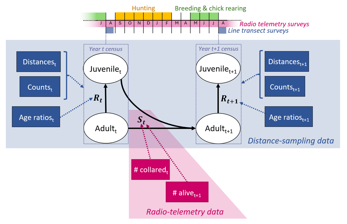
Figure 1 - Graphical representation of the annual ptarmigan life cycle with two age classes under a post-breeding census and the data sources included in the integrated distance sampling model. Solid arrows represent relationships within the ptarmigan life cycle; dotted arrows visualize information flow from data sources to parameters. Blue and pink data nodes originate from distance sampling and line transect surveys, respectively. Juvenilet = juveniles in year \(t\). Adultt = adults in year \(t\). \(R_{t}\) = recruitment rate in year \(t\). \(S_{t}\) = survival probability from year \(t\) to \(t + 1\).
Likelihoods for distance sampling data
The implementation of the modelling framework we present assumes that the distance sampling survey data have the following characteristics: 1) the survey consists of line transects, 2) animals may be detected alone or in groups, and 3) juveniles and adults can be distinguished during surveys. These characteristics are inspired by our willow ptarmigan case study (details below). Our model includes three likelihoods for different components of the age-structured distance sampling data. First is the likelihood for the perpendicular detection distances from line transect, \(y\), which are linked to distance-dependent detection probability \(p_{y}\) through a half-normal detection function:
\(p_{y} = \exp\left( - \frac{y^{2}}{2\sigma^{2}} \right)\)
where \(\sigma\) is the half-normal detection parameter. We assumed \(\sigma\) to vary among years (index \(t\)) but not between transect lines or animal group sizes. Following Moore and Barlow (2011), the resulting \(\sigma_{t}\) can be used to calculate effective strip width (\(esw_{t}\)) and, consequently, average detection probability per line transect with a truncation distance \(W\) (i.e. the distance in meter beyond which observations are discarded) according to:
\(\begin{matrix} esw_{t} & = \sqrt{\frac{\pi*\sigma_{t}^{2}}{2}} \\ \widehat{p_{t}} & = esw_{t}/W \end{matrix}\)
The estimated average detection probability \(\widehat{p_{t}}\) is an integral part of the second data likelihood which relates the observed number of animals in each age class \(a\), \(obsN_{a,j,t}\) (\(j\) = transect) to the corresponding true number per transect, \(N_{a,j,t}\):
\(obsN_{a,j,t} \sim Poisson\left( \widehat{p_{t}}*N_{a,j,t} \right)\)
\(N_{juv,j,t}\) and \(N_{ad,j,t}\) are then linked back to the population model by converting them to densities through multiplication by \(2L_{j,t}W\) (where \(L_{j,t}\) is length of transect \(j\) in year \(t\), and \(W\) is the truncation distance).
The third data likelihood focuses on the counts of adults (\(obsAd_{j,t}\)) and juveniles (\(obsJuv_{j,t}\)) observed during the distance sampling surveys and links them to the estimated year-specific recruitment rate:
\(obsJuv_{j,t} \sim Poisson\left( \widehat{R_{t}}*obsAd_{j,t} \right)\)
Likelihood for radio-telemetry data
The final likelihood is for the auxiliary telemetry data. It is set up under the assumption of perfect detection, and hence known fates, of animals bearing transmitters and links the numbers of animals released at the start of season \(k\) of year \(t\) to the number of survivors at the end of the same season:
\(survivors_{k,t} \sim Binomial\left( released_{k,t},\widehat{Sk_{t}} \right)\)
Here, \(\widehat{Sk_{t}}\) is the survival probability over the relevant time interval \(k\) in year \(t\). The length and definition of \(k\) will be specific to any given study. For the remainder of this article, we define \(k\) as 6-month seasons to be consistent with our ptarmigan case study. Consequently, the annual survival probability, \(S_{t}\) that appears in the population model above is calculated as the product of two seasonal survival probabilities, \(S1_{t}\) defined as survival probability from August through January, and \(S2_{t}\) defined as survival probability from February through July.
Hierarchical models with time-variation in parameters
Vital rates (survival probabilities \(S_{t}\), recruitment rates \(R_{t}\)) and detection parameters (half-normal detection parameters \(\sigma_{t}\)) can all be modelled as time-dependent in our framework. For both the tests with simulated data and the case study described below, we implemented log-normally distributed random year effects on recruitment rate and detection probability. In the case study, we additionally included a covariate effect (see details below) on log recruitment rates, resulting in the following model:
\(\log\left( R_{t} \right) = \log\left( \mu_{R} \right) + \beta*cov_{t} + \epsilon_{t}\)
\(\mu_{R}\) represents the mean recruitment rate if the covariate \(cov_{t}\) is centered around 0 (e.g. z-standardized) or a baseline recruitment rate corresponding to \(cov_{t} = 0\) if the covariate is not centered. \(\beta\) the slope of the covariate effect, and \(\epsilon_{t}\) the normally distributed random effects.
In both simulations and the case study, we treated survival as time-invariant. This was motivated by our case study: previous research has relatively low interannual variation in survival of our focal ptarmigan population (Israelsen et al. 2020) and the telemetry data used in this study has limited potential for accurately estimating time-variation as it is relatively sparse. We note, however, that also survival could be modelled as time-dependent if sufficient data is available.
Model testing with simulated data
We assessed the model’s overall performance and ability to estimate abundance, demographic rates, and detection parameters without bias by testing it on simulated data. We generated a total of 10 simulated datasets in five steps. First, we simulated 15-year time-series of survival and recruitment rates from biologically plausible values for averages and – in the case of recruitment – among-year variation in demographic rates (survival was held constant across years). Second, we used the yearly demographic rate and realistic initial population densities to simulate stochastic population dynamics in 50 distinct sites. Third, we simulated the grouping of individuals in each site by first determining the expected number of groups in a site (based on the average group size of 5.6 from our ptarmigan data) and then distributing individuals among groups via multinomial trials. Fourth, we assigned a distance from transect line to each group and simulated the line transect survey in all 50 sites across 15 years. Finally, we simulated 5-year time-series of radio-telemetry data (= survival from one year to the next) for a subset of individuals (30 per year on average) using the simulated survival probabilities for each relevant year. We then fit the IDSM to each of the 10 simulated datasets three times, using distinct seeds for both simulating initial values and initiating and running the MCMC. Model implementation for simulated data tests was largely identical to that for real data and is described in detail below. For assessing model performance, fit, and bias, we 1) compared model estimates to the true values of parameters used for data simulations visually, 2) correlated estimated and true values, and 3) calculated two metrics to measure bias: the proportion of samples above the true value (corresponding to Bayesian p-values) and the root-mean square deviation (RMSD).
Case study
To demonstrate the applicability of the IDSM to real data, we applied it to a case study of willow ptarmigan, a small grouse species with a has a circumpolar distribution (Fuglei et al., 2020). In Norway, there has been a long-term decline in willow ptarmigan abundance across more than a century (Hjeljord and Loe 2022), but in the last few decades abundance trends have fluctuated substantially both across time and space. Willow ptarmigan is a valued game species (Andersen et al. 2014), and there have been several long-term research projects devoted to understanding how they respond to environmental variation and harvest management (Israelsen et al. 2020; Sandercock et al. 2011). A key insight from across several study areas is the annual recruitment rate (i.e. \(R_{t}\) in our model, as outlined above) is highly variable, and is affected both by spring conditions (Eriksen et al. 2023) and the abundance of small rodents, which constitute alternative prey for common predators (i.e. the Alternative Prey Hypothesis, see Hagen 1952; Kausrud et al. 2008; Bowler et al. 2020). Adult survival show less inter-annual fluctuations (Israelsen et al. 2020), although variation due to e.g. harvest management is evident when comparing across studies (Israelsen et al. 2020; Sandercock et al. 2011).
Our case study was based on an ongoing long-term research project on willow ptarmigan in Lierne municipality in Central Norway (approximately 62.4 degrees north and 13.2 degrees east). The study area is located in a sub-alpine ecosystem, and the landscape is a mosaic of open heath and shrub vegetation (dominated by Ericacea, willow shrub Salix spp., and dwarf birch Betula nana), interspersed with bogs and forest patches (mainly birch Betula spp.). The climate is strongly seasonal, with snow typically covering the ground from October/November through April/May.
From this study system, two datasets were used for the case study:
Data from a line transect survey program targeting willow ptarmigan operated under the natural resources management authorities (2007-2021, ongoing)
Data from an individual-based monitoring programme based on radio collared willow ptarmigan (2015-2021, ongoing)
Line transect survey data were collected in August each year, prior to the annual autumn harvest season, as part of the program “Hønsefuglportalen”. Hønsefuglportalen is a national program for line transect surveys of tetraonid birds, and the effort is directed mainly towards willow ptarmigan habitats. In our case study, we used data from the western part of Lierne municipality. Line transects are surveyed by trained volunteers that use pointing dogs to locate the birds. When located, the geographical coordinate, perpendicular distance from the sampling line, the number of birds in the group, as well as the age (juvenile or adult) and sex of the birds are recorded. As the surveys are conducted in early August, juveniles can be distinguished from adults by their smaller body size. Males and females are mainly distinguished by sound (males often make a characteristic sound when being flushed). Observers are trained to distinguish age classes and sexes, but incomplete identification can occur. In this application we assumed that the resulting “unknown” age and/or sex class birds were in fact juveniles (see discussion for further considerations). Besides bird observations, field workers also record whether (1) or not (0) they encounter small rodents on any transect line, allowing the proportion of transect lines with small rodent detection to be used as measure of rodent occupancy (covariate ranging from 0 to 1). After data are collected they undergo quality control, get standardized based on the Darwin-Core standard (Wieczorek et al. 2012), and made publicly available as a sampling-event data set published through GBIF (Nilsen et al. 2023). For additional description of the data collection procedures, see Bowler et al. (2020), Kvasnes et al. (2018) and Nilsen et al. (2023).
The radio-telemetry data is the result of an individual-based longitudinal study over the period 2015-2021. Each winter (in February-March), willow ptarmigan were located at night using snowmobiles and large hand nets with prolonged handles, as described in (Israelsen et al. 2020). High-powered head lamps were used to dazzle the birds and allow capture. Captured birds were fitted with a uniquely numbered leg ring (~ 2.4g) and a Holohil RI-2BM or Holohil RI-2DM radio transmitter (~ 14.1g) and subsequently released. The radio transmitters had an expected battery lifetime of 24 months (RI-2BM) or 30 months (RI-2DM), and included a mortality circuit that was activated if a bird had been immobile for 12 hours. We monitored the birds throughout most of the year by triangulation from the ground at least once a month for 10 months of the year (February – November) by qualified field personnel. A number of birds dispersed out of the main study areas and was thus out of signal range for field personnel on the ground. To avoid loss of data, we conducted aerial triangulation using a helicopter or airplane three times a year (May, September and November) in the years 2016-2020. In the analysis here, we assume that the telemetry data is representative for the entire duration of study period (2007-2021), despite its collection only starting in 2015. Data on marked birds were collected with highest concern to animal welfare, under legal authorisation from the Norwegian Food Safety Authority (IDs 8477, 15166 and 22919).
Bayesian model implementation
We implemented the model in a Bayesian framework using NIMBLE version 1.0.1 (de Valpine et al. 2017) in R version 4.3.1 (R Core Team 2023). The likelihood for line transect observation distances was set up using a custom half-normal distribution developed by Michael Scroggie as part of the “nimbleDistance” package (https://github.com/scrogster/nimbleDistance). We used non-informative uniform priors (with biologically reasonable boundaries where possible) for all parameters. We assumed constant survival and time-varying recruitment rate in models fit to both simulated and real data.
For the model fits to simulated and real data we ran 3 (simulated) or 4 (real) MCMC chains with NIMBLE’s standard samples for 100k iterations. 40k thereof were discarded as burn-in prior to thinning with factor 20, leaving us with 3k posterior samples per chain (total of 12k samples per run). MCMC parameters were chosen to yield a representative number of samples from converged chains, and convergence was determined based on visual inspection of trace plots. Posterior samples from the model fitted to real data are available at Nilsen and Nater (2024) (in folder PosteriorSamples_LierneCaseStudy).
Results
Model performance on simulated datasets
Models fit to simulated datasets reached MCMC convergence within the implemented 100k iterations. Chain mixing was good for all parameters except average recruitment rate (\(\mu_{R}\)); for this parameter, an elevated degree of autocorrelation was visible in the MCMC chains in some of the replicate runs, but models still produced posterior distributions that well represented the true value used in simulations (Figure 2).
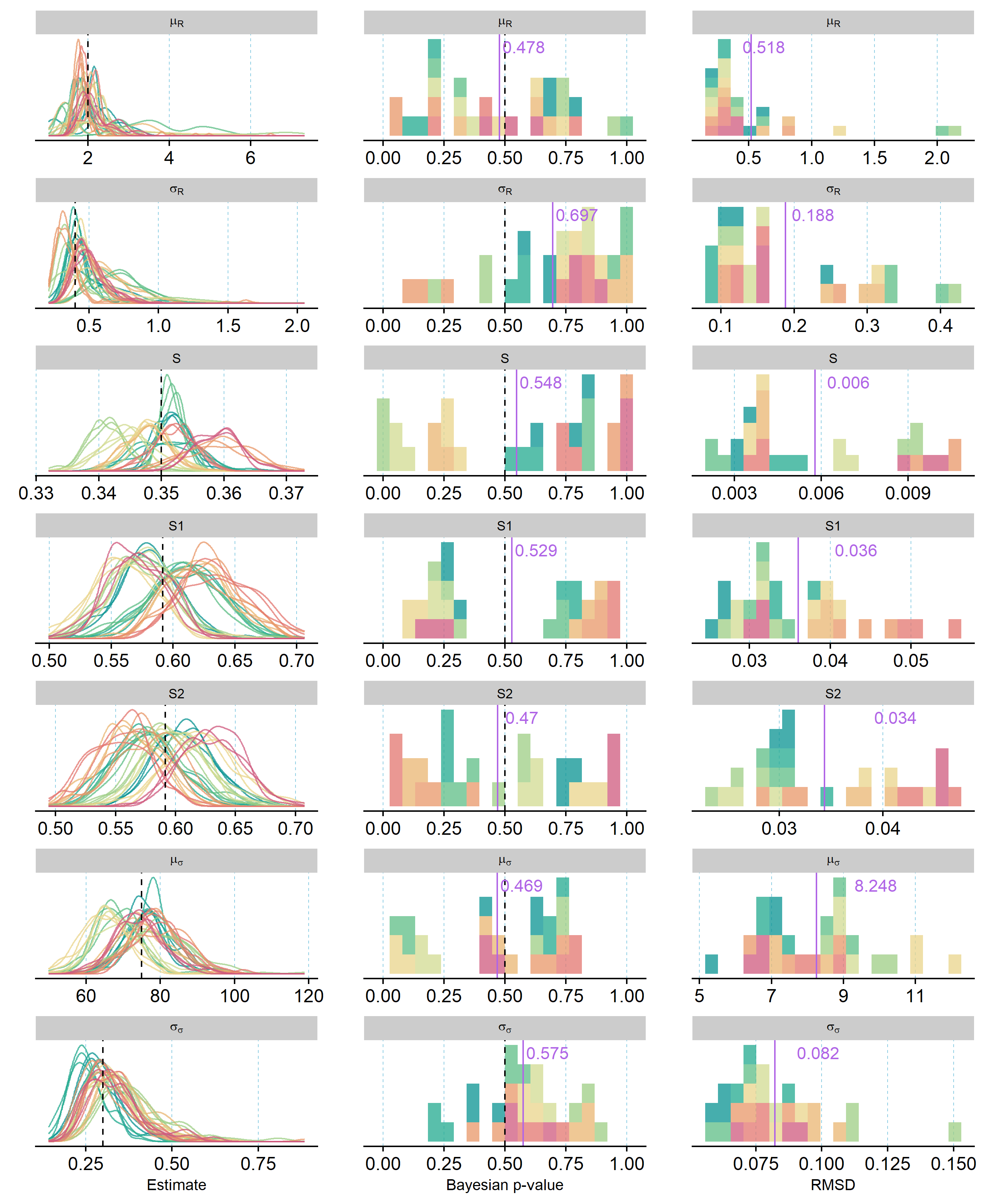
Figure 2 - Vital rate and detection parameter averages estimated from 10 distinct sets of simulated data (= colors) using three model fits each. First columns depicts posterior densities from each model run relative to the true value used to simulate data (black dashed line). Second and third columns visualize the distributions of Bayesian p-values (proportion of samples > true value) and root-mean square deviations (RMSD) for all model runs, respectively. Purple lines and numbers mark the mean values across all model runs; dashed black line (second row only) marks the ideal Bayesian p-value of 0.5.
Posterior estimates relative to true values, Bayesian p-values, and RMSD for parameters estimated in three model fits to each of 10 simulated data sets are shown in Figure 2 and Figure 3. Overall, the IDSM was able to correctly estimate the majority of parameters from all 10 simulated datasets without substantial systematic bias. The replicate runs for each dataset resulted in very similar posterior distributions, demonstrating that the models converged towards the same posterior distributions irrespective of starting values. This may not seem to be the case for survival parameters (Figure 2), but this is largely due to the relatively low number of individuals in the simulated telemetry data; estimated posteriors match up well with simulated numbers of survivors in each datasets, and the averages of Bayesian p-values fell very close to 0.5 (= no bias). For time-variation in recruitment rate (\(\sigma_{R}\)), on the other hand, the average Bayesian p-value indicated a potential for overestimation (p = 0.697), and this is consistent with the relatively large spread of Bayesian p-values for year-specific recruitment rates (Figure 3). Across all years, the correlation between predicted and true recruitment rates was very high, yet closer inspection showed that slight over- and under-estimation was present for certain years across all replicates (see supplementary figures in folder SimCheck_byDataSet in Nilsen and Nater (2024)). This was also the case for year-specific estimates of population density and detection probability, but both were slightly more likely to be underestimated than overestimated (Figure 3).
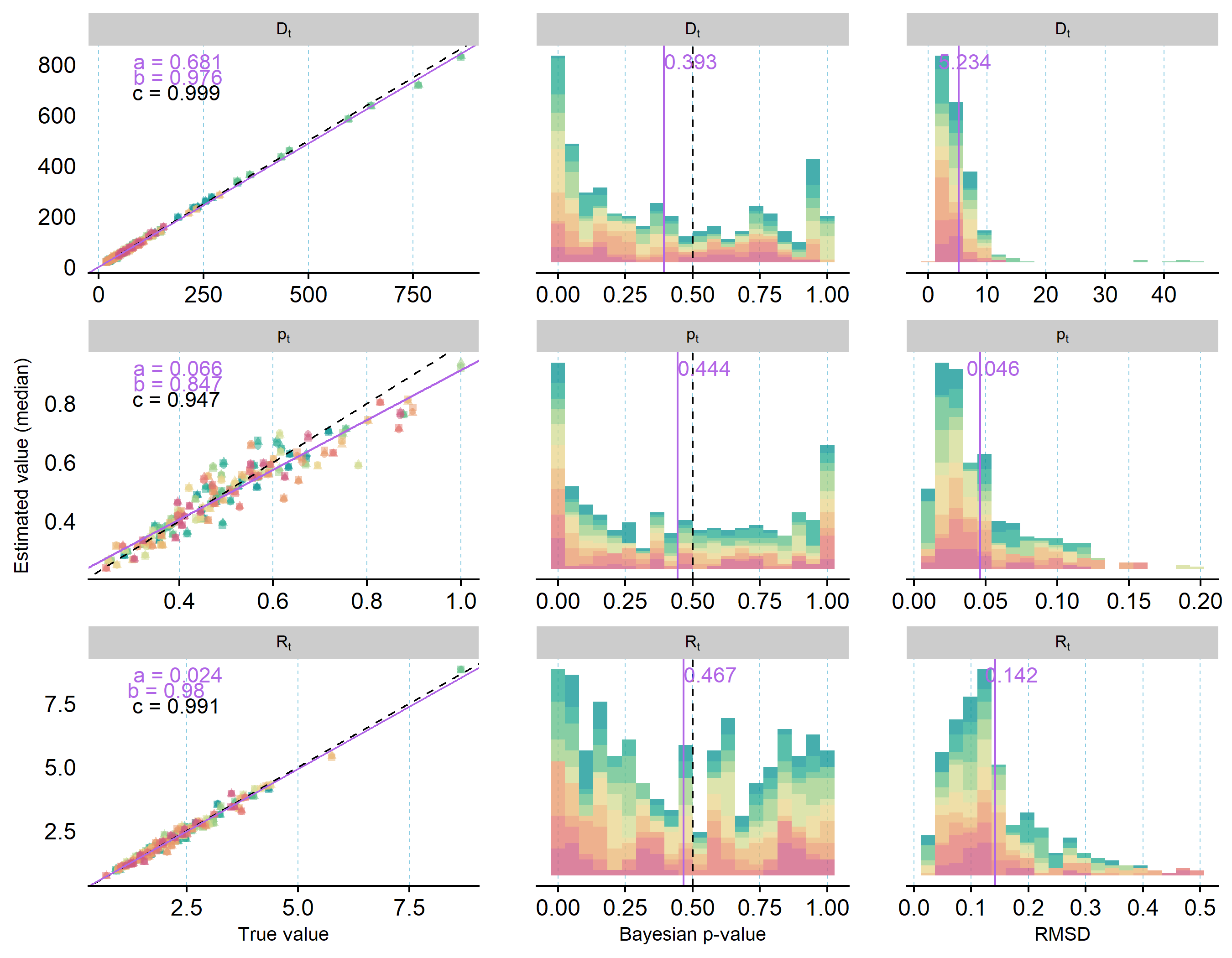
Figure 3 - Annual population density (\(D_{t}\)), detection probability (\(p_{t}\)), and recruitment rate (\(R_{t}\)) estimated from 10 distinct sets of simulated data (= colors) using three model fits each. First column depicts the relationship between posterior medians from each model run and the true value used to simulate data (purple solid line = relationship estimated from linear model with a = intercept and b = slope; black dashed line = perfect correlation; c = estimated correlation coefficient). Second and third columns visualize the distributions of Bayesian p-values (proportion of samples > true value) and root-mean square deviations (RMSD) for all model runs, respectively. Purple lines and numbers mark the mean values across all model runs; dashed black line (second row only) marks the ideal Bayesian p-value of 0.5. And equivalent figure showing posterior samples instead of posterior means is available in the supplementary material on OSF.
Case study on willow ptarmigans in Central Norway
Having evaluated the overall performance of our model on simulated data, we used data from our case study in Lierne to estimate abundance, vital rates and detection probabilities from a real-world data set. Like the model fits to simulated data, convergence was reached within the given amount of iterations and mixing was good, albeit with somewhat higher chain autocorrelation for the intercept in the recruitment model. Ptarmigan population density was estimated with a marked increase across the study period, from < 10 ptarmigan / \(km^{2}\) in 2007 to > 35 ptarmigan / \(km^{2}\) in in 2021 (Figure 4). The increase was most distinct from 2016 and onward.
The average probability of detecting individuals and groups of ptarmigan within transect line areas was 0.61 (95% C.I = 0.57 - 0.65), and estimated with a detection decay parameter \(\sigma\) of 95.3 (95% C.I = 82.18 - 110.43). Detection probabilities were highest in the start of the study and in the period 2016-2019 and lowest from 2010-2012. The relationship between detection probability and distance and changes in detection over time are visualized in supplementary figures “DetectionProb_distance.png” and “TimeSeries_pDetect.png” in Nilsen and Nater (2024).
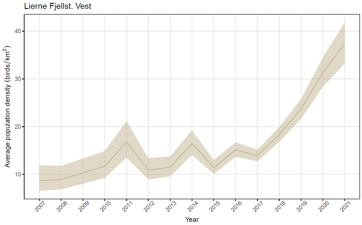
Figure 4 - Estimated density of willow ptarmigans in Lierne from 2007 to 2021. Solid line represents the posterior median, ribbon marks 95% credible interval.
Average survival probability for August - January (\(S_{1}\)) was estimated at 0.46 (95% C.I = 0.42 - 0.5) while average survival probability for February - July (\(S_{2}\)) was estimated as 0.64 (95% C.I = 0.59 - 0.7) (Figure 5 A). Annual survival probability \(S\), given by the product of \(S_{1}\) and \(S_{2}\), was estimated at 0.3 (95% C.I = 0.29 - 0.31), Figure 5 A).
Recruitment (\(R_{t}\)) was allowed to vary across years (see model specification), and estimates displayed large inter-annual variability (Figure 5 C, Figure S1). While the mean (baseline) recruitment \(\mu_{R}\) was estimated as 2.7 (95% C.I = 2.3 - 3.2) the yearly recruitment rates ranged from 1.2 in year 2012 to 4.9 in year 2007.
Given the available data, the IDSM was not able to estimate a clear effect of small rodent abundance on ptarmigan recruitment (slope-parameter for the z-standardized rodent occurrence data = 0.062 ; 95% C.I. = -0.2 - 0.31, see supplementary figure “Rep_betaR.R.png” in Nilsen and Nater (2024)).
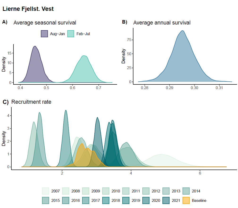
Figure 5 - Posterior densities of A) seasonal survival, B) average annual survival, and C) recruitment rate. For the latter, the yellow distribution is for the intercept, representing a baseline recruitment rate when rodent occupancy is low. The turquoise distributions are for year-specific estimates or recruitment rate, with darker colors indicating later years. For a visualization of the time-series of recruitment rates, see supplementary figure “TimeSeries_rRep” on OSF.
Discussion
We developed an integrated population model that jointly analyses line transect distance sampling survey data and data from marked individuals to estimate population abundance, survival probabilities, and recruitment rates over time. We first used simulated data to examine the model’s ability to retrieve the underlying parameters when they were known. We then fitted the model to data from an ongoing field study on willow ptarmigan in Norway to showcase its applicability to real wildlife monitoring data.
Open population formulations of the distance sampling model have previously been presented and applied to various ecological systems (Sollmann et al. 2015; Bowler et al. 2020; Moore and Barlow 2011). The model presented here extends those previous applications by formulating the underlying population process model as a stage-structured matrix model (Caswell 2000) in which the matrix elements are represented by annual survival probabilities and recruitment rates. While this has been the common approach for a range of other statistical modelling frameworks, including the growing suite of models falling into the category of integrated population models (Schaub and Kéry 2021), the integration of mechanistic population models into distance sampling frameworks is rather new. The resulting modelling framework allow us to make maximum use of distance sampling data in combination with auxiliary information both from the distance sampling survey itself (i.e. information on age, sex, etc. of observed animals) and from other types of monitoring, and enables estimation not only of changes in population density but also of underlying vital rates over time.
In general, the model did a good job at recreating the underlying parameters when fitted to simulated data with known underlying true parameter values. The simulated data sets were based relatively wide ranges of parameter values, yet model posteriors included the true values in almost all cases. While there seems to be potential for overestimating time variation in recruitment rates, this bias did not propagate into estimates of year-specific recruitment rates (Figure 3), and may be related to the subpar mixing of the intercept of the recruitment model. The model was more likely to under- than overestimate detection probabilities and population densities, but bias in these estimates was generally small and spread out across time-series, i.e. bias did not seem to arise disproportionately at e.g. the starts or ends of time-series. Simulated data tests also revealed that telemetry data simulated with an average of 30 individuals may be too sparse to obtain robust and generalisable estimates of seasonal survival probabilites. This could be investigated further by repeating simulated data runs with different average numbers of individuals in the telemetry data, but we chose not to go down this path here as we were primarily interested in model performance given the amounts of data that are currently available for our ptarmigan case study. Based on the simulated data tests presented here, we conclude that the IDSM is able to provide meaningful and sufficiently accurate and robust estimates of demographic parameters from age-structured distance sampling data, provided that the input data are unbiased (with respect to the underlying model formulation).
Real data, however, are likely to be subject to certain biases, which may result in biased parameter estimates unless accounted for. One type of bias that is likely to be common for age-structured distance sampling data arises from failure to (correctly) classify the age class of observed individuals. In our case study on willow ptarmigan in Norway, such misclassification is likely to happen at an unknown rate, even if the size difference between adult and juvenile birds are quite substantial during the survey. Moreover, The probability for misclassificiation might be related to both the timing of the survey (e.g. mid August rather than early August), it might vary between observers, and even by survey conditions. Observations with incorrectly classified age have the potential to introduce bias in the IDSMs relative estimates of survival and recruitment. This is due to the way it uses the distance sampling data to estimate survival and recruitment rates. In our process model, the population growth rate (\(\lambda\)) is determined by the survival and recruitment rate in the following way: \(\lambda = S + (S*R)\), and this creates a dependence between the demographic parameters. If the age ratio in the data are biased or contain frequent misclassifications, this is likely to affect the relative contribution of survival and recruitment to the growth rate. To get an idea of the potential effect of this on parameter estimation, we checked the sensitivity of the output of the model fit to real data with regard to the treatment of birds classified as “unknown sex and age” by the field personnel (see Methods). In the model version presented in the results section, we made the assumption that these birds were in fact juveniles. Comparing estimates to an alternative scenario in which we discarded all birds classified as “unknown sex and age” (see supplementary figures in Nilsen and Nater (2024)) we found that – as expected – estimated population density was virtually unaffected by the treatment of “unknown sex and age” observations, while the annual demographic parameters shifted proportional to the amount of “unknown sex and age” observations in the given year (towards higher recruitment and lower survival). Thus, biases in the reported age ratios may affect estimations of demographic rates, but not so much population density. Since the proportion of “unknown sex and age” observations in our ptarmigan case study was low (< 3% of observations), potential biases in estimates resulting from age misclassification are expected to be small. Nonetheless, future developments of the IDSM modelling framework should focus on ways of accounting explicitly for misclassification of age class in the field.
The density estimates that we derived from the case study on Willow ptarmigan in Norway is comparable to previous estimates from across Norway (see e.g. Sandercock et al. 2011; Kvasnes et al. 2014a). Throughout the study period from 2007 - 2021, the density increased markedly, but the reason for this increase is not known. Compared to previous studies on ptarmigan (see e.g. Israelsen et al. 2020; Sandercock et al. 2011), we could have expected somewhat higher estimates of survival probability. One potential reason for the overall lower estimates obtained here is that our IDSM analysis assumed constant survival over the period 2007-2021 while survival, in reality, may have changed over time. If survival in more recent years, when telemetry data was collected (and the study of e.g. Israelsen et al. 2020 was carried out) was higher than in earlier years – something that seems likely given population increase over recent years – an average over the entire time period is expected to be lower. On a different note, we can also not exclude the possibility of a small degree of bias in survival estimates due to misclassification of age in the data (see above), especially seeing as the IDSM’s recruitment rate estimates also appear somewhat high compared to other studies on willow ptarmigan (Eriksen et al. 2023; Kvasnes et al. 2014b; Steen et al. 1988). As the ptarmigan case study served as an illustrative example for the IDSM framework in this article, we did not further investigate alternative models, such as implementations with time-varying survival or different treatment of uncertainty in age and/or sex. The model lends itself easily to such extensions, however, and methods such as posterior predictive checks and WAIC will be useful for assessing and optimizing the fit of the model to data from relevant case studies (Hooten and Hobbs 2015; Conn et al. 2018).
In addition to estimating demographic rates from line transect data, the IDSM also allows including relevant environmental effects on the demographic rates themselves, and not just on population growth rate as a whole (\(\lambda\)). In the ptarmigan case study we thus attempted to investigate the effect of small rodent abundance (approximated as the proportion of transect lines on which rodents were reported each year) on recruitment rate. We were not able to detect a clear effect of rodent abundance due to large uncertainty associated with the estimate (see Supplementary Figures “Rep_betaR.R.png” in Nilsen and Nater (2024)). This may seem somewhat surprising given that such a pattern has been reported repeatedly in the literature (see e.g. Bowler et al. 2020). We speculate that there are at least three potential and not mutually exclusive explanations to this result. The first is that our covariate data may not have been well suited for estimating effects on recruitment. The data on rodent abundance was zero-inflated, and the annual variation in the index was rather small otherwise, making for a covariate with relatively little information content. While this may be partially a consequence of how these data are collected, it is also well known that the amplitude and regularity of the rodent cycles has been fading in recent decades (Kausrud et al. 2008; Cornulier et al. 2013), and our study area might be no exception. Similar patterns have been seen in other rodent data sets collected from this region (Nilsen, E.B., pers obs). Lack of peak rodent years in the time series to which we fitted the model may thus also have contributed to making effect estimation challenging. Second, it is possible that rodent effects were obscured by other, potentially stronger, covariate effects. Previous research has shown that ptarmigan recruitment is also sensitive to the weather in the late winter and spring (before and during the breeding season); as we did not fit any weather covariates to the model, there is a possibility that effects of spring conditions in certain years may have masked any remaining effects of small rodent abundance. Finally, the data set used in this analysis is relatively short (15 years), leaving us with somewhat limited statistical power to detect effects of temporal covariates. Taken together we therefore do not consider this study as a particularly strong test of the underlying effect of small rodent fluctuations on ptarmigan recruitment rates. It is worth noting that future applications could increase statistical power by including either more years of data or capitalizing on space-for-time substitution as the Norwegian ptarmigan monitoring programme spans many more locations beyond Lierne. Bowler et al. (2020), for example, used data from the same sampling program but from more areas using a simpler open population DS model, and detected a very clear signal from small rodent abundance on ptarmigan population growth rate. An extension of our IDSM to include data from multiple areas therefore constitutes a promising approach for investigating to which extent similar results emerge by linking environmental covariates to the actual demographic rates and not only just to the resulting population growth rates.
The new IDSM framework presented here is relevant for many wildlife populations that are surveyed using line transect sampling that includes additional information on age, sex, and/or life stages of the observed individuals. Following the integrated modelling philosophy, the IDSM also allows for the integration of auxiliary data. In our application here, we integrated data from radio-telemetry of marked birds, which explicitly supported the estimation of survival probabilities. The IDSM framework is very flexible, however, and open to the inclusion of additional/other auxiliary data that contains information on demographic rates or population size/density. Moreover, the hierarchical nature of the model makes is straightforward to adapt to different species and to include different suites of environmental covariates on the demographic rates. Finally, it constitutes a modelling framework that is well suited for extension to multiple areas and thus able to capitalize on space-for-time substitution (Lovell et al. 2023) to produce large-scale and spatially explicit estimates of population density, demographic rates, and environmental effects from large-scale (participatory) monitoring.
Author contributions
Erlend B. Nilsen: Conceptualization, Methodology, Software, Formal analysis, Investigation, Data Curation, Writing - Original Draft, Writing - Review & Editing, Project administration, Funding acquisition.
Chloé R. Nater: Conceptualization, Methodology, Software, Validation, Formal analysis, Investigation, Data Curation, Writing - Original Draft, Writing - Review & Editing, Visualization.
Acknowledgements
We are grateful to field workers that collected the line transect data through the Hønsefuglportalen program. Fjellstyrene i Lierne and many colleagues from NINA and Nord University contributed both to the line transect program and the field work related to the marked willow ptarmigan. We also thank James A. Martin for constructive discussions during the later stages of this work and Simon Hansul, Tiago Marquez, and Sandrine Charles for constructive feedback on the manuscript during the review process.
Preprint version 3 of this article has been peer-reviewed and recommended by Peer Community In Peer Community in Ecology (https://doi.org/10.24072/pci.ecology.100642; Charles, 2025).
Funding
Both data collection and analytical work were financed by the Norwegian Environment Agency funded the projects (grant nrs 17010522, 19047014 and 22047004).
Conflict of interest disclosure
The authors declare that they comply with the PCI rule of having no financial conflicts of interest in relation to the content of the article.
Data and code availability
The raw data from the line transect surveys is deposited on GBIF and can be accessed freely via the Living Norway Data Portal (https://data.livingnorway.no). The work here is based on version 1.7 of the dataset “Tetraonid line transect surveys from Norway: Data from Fjellstyrene” (https://doi.org/10.15468/975ski; Nilsen et al. 2023).
The auxiliary radio-telemetry data and rodent occupancy data, all code used for wrangling, analysing, and visualizing data and results, as well as vignettes providing rich text documentation of all steps in the workflows for simulated and real data analysis, can be found in the project’s repository on GitHub: https://github.com/ErlendNilsen/OpenPop_Integrated_DistSamp. The results presented in this paper were created using version 1.5 of the code (https://doi.org/10.5281/zenodo.13627743; Nater et al. 2024).
Supplementary figures and posterior samples from the model run on the real data are available as a time-stamped open archived on Open Science Framework (https://doi.org/10.17605/OSF.IO/TPRV2; Nilsen and Nater 2024).